The gamlss.prepdata package originated from the gamlss.ggplots package. As gamlss.ggplots became too large, for easy maintenance, it was split into two separate packages, and gamlss.prepdata was created.
Since gamlss.prepdata is still at an experimental stage, some of functions are remained hidden to allow time for thorough checking and validation. These hidden functions can still be accessed using the triple colon notation, for example: gamlss.prepdata:::.
The functions available in gamlss.prepdata are intended for pre-fitting — that is, to be used before applying the gamlss() or gamlss2() fitting functions. The available functions can be grouped into the following categories:
Information functions
These functions provide information about:
the size of the dataset;
the extent of missing values;
the structure of the dataset;
whether the class of variables is appropriate for analysis.
Plotting functions
These functions allow plotting;
individual variables and
pairwise relationships of variables
Features functions
These functions can assist in:
detecting outliers;
applying transformations to variables and
scaling variables.
Data Partition functions
Functions that facilitate partitioning the data to improve inference and avoid overfitting during model selection.
Distributional Regression
The aim of this vignette is to demonstrate how to manipulate and prepare data before applying a distributional regression analysis.
The general form a distributional regression model can be written as; \[
\begin{split}
\textbf{y} & \stackrel{\small{ind}}{\sim } \mathcal{D}( \boldsymbol{\theta}_1, \ldots, \boldsymbol{\theta}_k) \nonumber \\
g_1(\boldsymbol{\theta}_1) &= \mathcal{ML}_1(\textbf{x}_{11},\textbf{x}_{21}, \ldots, \textbf{x}_{p1}) \nonumber \\
\ldots &= \ldots \nonumber\\
g_k(\boldsymbol{\theta}_k) &= \mathcal{ML}_k(\textbf{x}_{1k},\textbf{x}_{2k}, \ldots, \textbf{x}_{pk}).
\end{split}
\tag{1}\] where we assume that the response variable \(y_i\) for \(i=1,\ldots, n\), is independently distributed having a distribution \(\mathcal{D}( \theta_1, \ldots, \theta_k)\) with \(k\) parameters and where all parameters could be effected by the explanatory variables \(\textbf{x}_{1},\textbf{x}_{2}, \ldots, \textbf{x}_{p}\). The \(\mathcal{ML}\) represents any regression type machine learning algorithm i.e. LASSO, Neural networks etc.
When only additive smoothing terms are used in the fitting the model can be written as; \[\begin{split}
\textbf{y} & \stackrel{\small{ind}}{\sim } \mathcal{D}( \boldsymbol{\theta}_1, \ldots, \boldsymbol{\theta}_k) \nonumber \\
g_1( \boldsymbol{\theta}_1) &= b_{01} + s_1(\textbf{x}_{11}) + \cdots, +s_p(\textbf{x}_{p1}) \nonumber\\
\ldots &= \ldots \nonumber\\
g_k( \boldsymbol{\theta}_k) &= b_{0k} + s_1(\textbf{x}_{1k}) + \cdots, +s_p(\textbf{x}_{pk}).
\end{split}
\tag{2}\] which is the GAMLSS model introduced by Rigby and Stasinopoulos (2005).
For all factors in the data the first level becomes the level with lower of higher number of observations
Next we demonstrate simple use of the functions.
data_dim()
This function provides detailed information about the dimensions of a data.frame. It is similar to the R function dim(), but with additional details. The output is the original data frame, allowing it to be used in a series of piping commands.
rent99 |>data_dim()
**************************************************************
**************************************************************
the R class of the data is: data.frame
the dimensions of the data are: 3082 by 9
number of observations with missing values: 0
% of NA's in the data: 0 %
**************************************************************
**************************************************************
If the variables in the dataset have very long names, they can be difficult to handle in formulae during modelling. The function data_shorter_names() abbreviates the names of the explanatory variables, making them easier to use in formulas.
rent99 |>data_shorter_names()
**************************************************************
**************************************************************
the names of variables
[1] "rent"  "rents" "area"  "yearc" "locat" "bath"  "kitch" "cheat" "distr"
**************************************************************
**************************************************************
If no long variable names exist in the dataset, the function data_shorter_names() does nothing. However, when applicable, the function abbreviates long names and returns the original data frame with the new shortened names.
Warning
Note that there is a risk when using a small value for the max option, as it may result in identical names for different variables. This could lead to confusion or errors in the modelling process. It is important to carefully choose an appropriate value for max to avoid this issue.
The function data_omit() omits all observations with missing values.
rent99 |>data_omit()
**************************************************************
**************************************************************
the R class of the data is: data.frame
the dimensions of the data before omition are: 3082 x 9
the dimensions of the data saved after omition are: 3082 x 9
the number of observations omited: 0
**************************************************************
**************************************************************
The output of the function is a new data frame withll NA’s omitted.
Warning
It is important to select the relevant variables for the analysis before using the data_omit() function, as some unwanted variables may contain many missing values that that could lead to unnecessary omissions.
Often, variables in datasets are read as character vectors, but for analysis, they may need to be treated as factors. This function transforms any character vector (with a relatively small number of distinct values) into a factor.
rent99 |>data_cha2fac() -> da
**************************************************************
not character vector was found
Since no character were found nothing have changed. The output of the function is a new data frame.
There are occasions when some variables have very few distinct observations, and it may be better to treat them as factors. The function data_few2fac() converts (numeric) vectors with a small number of distinct values into factors.
rent99 |>data_few2fac() -> da
**************************************************************
    rent  rentsqm     area    yearc location     bath  kitchen cheating
    2723     3053      132       68        3        2        2        2
district
     336
**************************************************************
4 vectors with fewer number of values than 5 were transformed to factors
**************************************************************
**************************************************************
Occasionally, we need to convert integer variables with a very large range of values into numeric vectors, especially for plots. The function data_int2num() performs this conversion.
rent99 |>data_int2num() -> da
**************************************************************
    rent  rentsqm     area    yearc location     bath  kitchen cheating
    2723     3053      132       68        3        2        2        2
district
     336
2 integer vectors with more number of values than 50 were transformed to numeric
**************************************************************
Occasionally, we need to convert integer variables with a very large range of values into numeric vectors, especially for plots. The function data_int2num() performs this conversion.
da <-data_fac2num(rent, vars=c("B"))
**************************************************************
**************************************************************
the R class of the data is: data.frame
the dimensions of the data before omition are: 1969 x 9
the dimensions of the data saved after omition are: 1969 x 9
the number of observations omited: 0
**************************************************************
**************************************************************
For analysisng datasets, it’s easier to keep only the relevant variables. The function data_rm() allows you to remove unnecessary variables, making the dataset more manageable for analysis.
data_rm(rent99, c(2,9)) -> dadim(rent99)
[1] 3082 9
dim(da)
[1] 3082 7
The output of the function is a new data frame. Note that this could be also done using the function select() of the package dplyr, or our own data_select() function.
Occutionally when we read data from files in Rsome extra variables are accidentaly produced with no values but NA’s. The function data_rmNAvars() removes those variables from the data;
This function searches for variables with only a single distinct value (often factors left over from a previous subset() operation) and removes them from the dataset.
Searches for potential pairwise interactions between variables in the dataset to identify relationships or dependencies that may be useful for modelling
Plots the response variable against various power transformations of the continuous x-variables to explore potential relationships and model suitability
Next we give examples of the graphical functions.
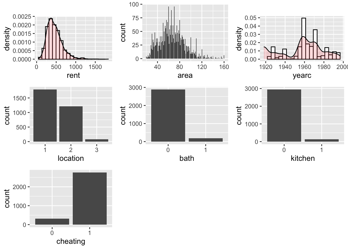
data_plot()
The function data_plot plots all the variables of the data individually; It plots the continuous variable as histograms with a density plots superimposed, see the plot for rent and yearc. As an alternative a dot plots can be requested see for an example in ?@sec-data_response. For integers the function plots needle plots, see area below and for categorical the function plots bar plots, see location, bathkitchen and cheating below.
da |>data_plot()
 100 % of data are saved,
that is, 3082 observations.
Warning: Removed 2 rows containing missing values or values outside the scale range
(`geom_bar()`).
Removed 2 rows containing missing values or values outside the scale range
(`geom_bar()`).
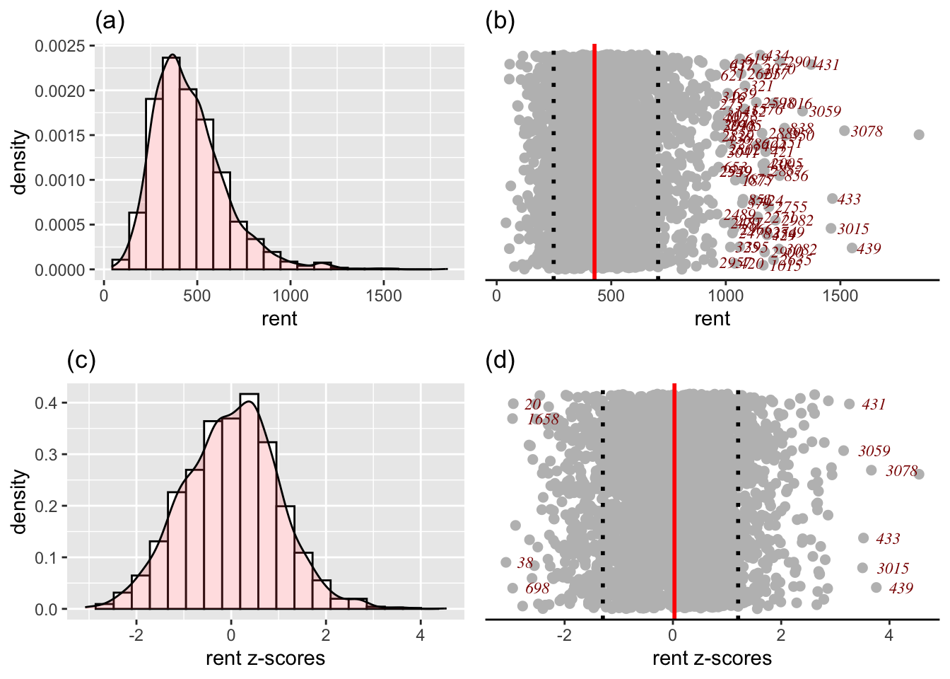
The function data_response() plots four different plots related to a continuous response variable. It plots; i) a histogram (and the density function); ii) a dot plot of the response in the original scale iii) a histogram (and the density function) of the response at the z-scores scale and vi) s dot-plot in the z-score scale.
The z-score scale is defined by fitting a distribution to the variable (normal or SHASH) and then taking the residuals, see also next section. The dot plots are good in identify highly skew variables and unusual observations. They display the median and inter quantile range of the data. The y-axis of a dot plot is a randomised uniform variable (therefore the plot could look slightly different each time.)
da |>data_response(, response=rent)
 100 % of data are saved,
that is, 3082 observations.
the class of the response is numeric is this correct?
a continuous distribution on (0,inf) could be used
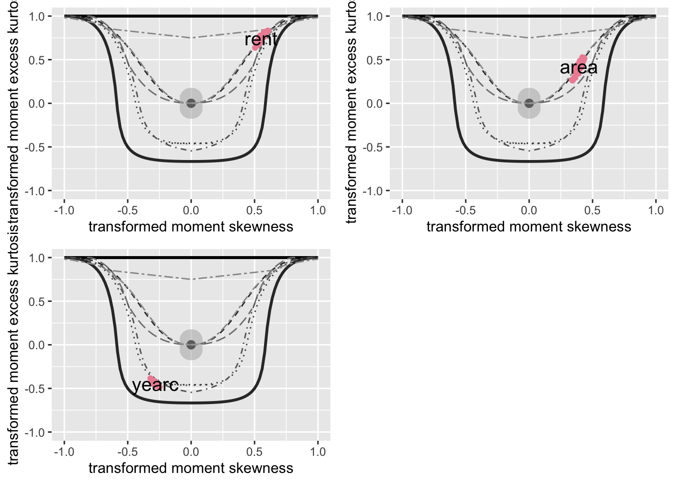
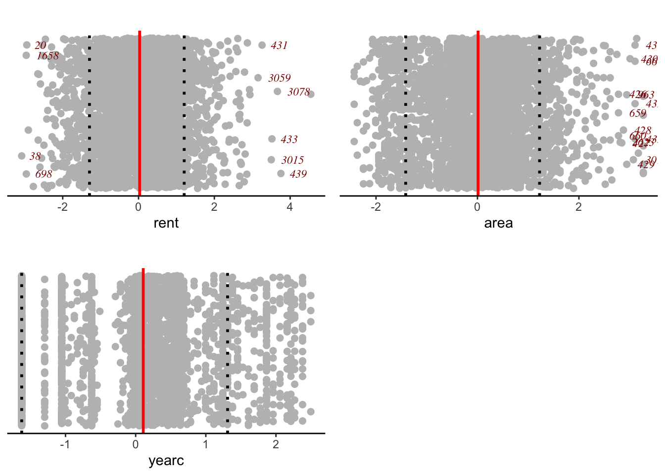
One could fit any four parameter (GAMLSS) distribution, defined on \(-\infty\) to \(\infty\), to any continuous variable, where skewness and kurtosis is suspected and take the quantile residuals (z-scores) as the transformed values of the x-values. The function y_zscores() performs just this. It takes a continuous variable and fits a continuous (four parameter SHASHo) distribution and gives the z-scores. The fitting distribution is specified by the user, but the default is SHASHo. The function data_zscores() takes all continuous variables and plots their z-scores. The methodology is use also to identify outliers in data_outliers().
da |>data_zscores()
 100 % of data are saved,
that is, 3082 observations.
In order to see how the z-scores are calculated consider the function y_zscores() which is taking an individual variables z-scores;
z <-y_zscores(rent99$rent, plot=FALSE)
The function is equivalent of fitting a constant model to all the parameters of a given distribution and than taking the quantile residuals (or z=scores) as he variable of interest. The default distribution is the four parameter SHASHo distribution.
library(gamlss2)m1 <-gamlssML(rent99$rent, family=SHASHo) # fitting a 4 parameter distribution cbind(z,resid(m1))[1:5,]# and taking the residuals
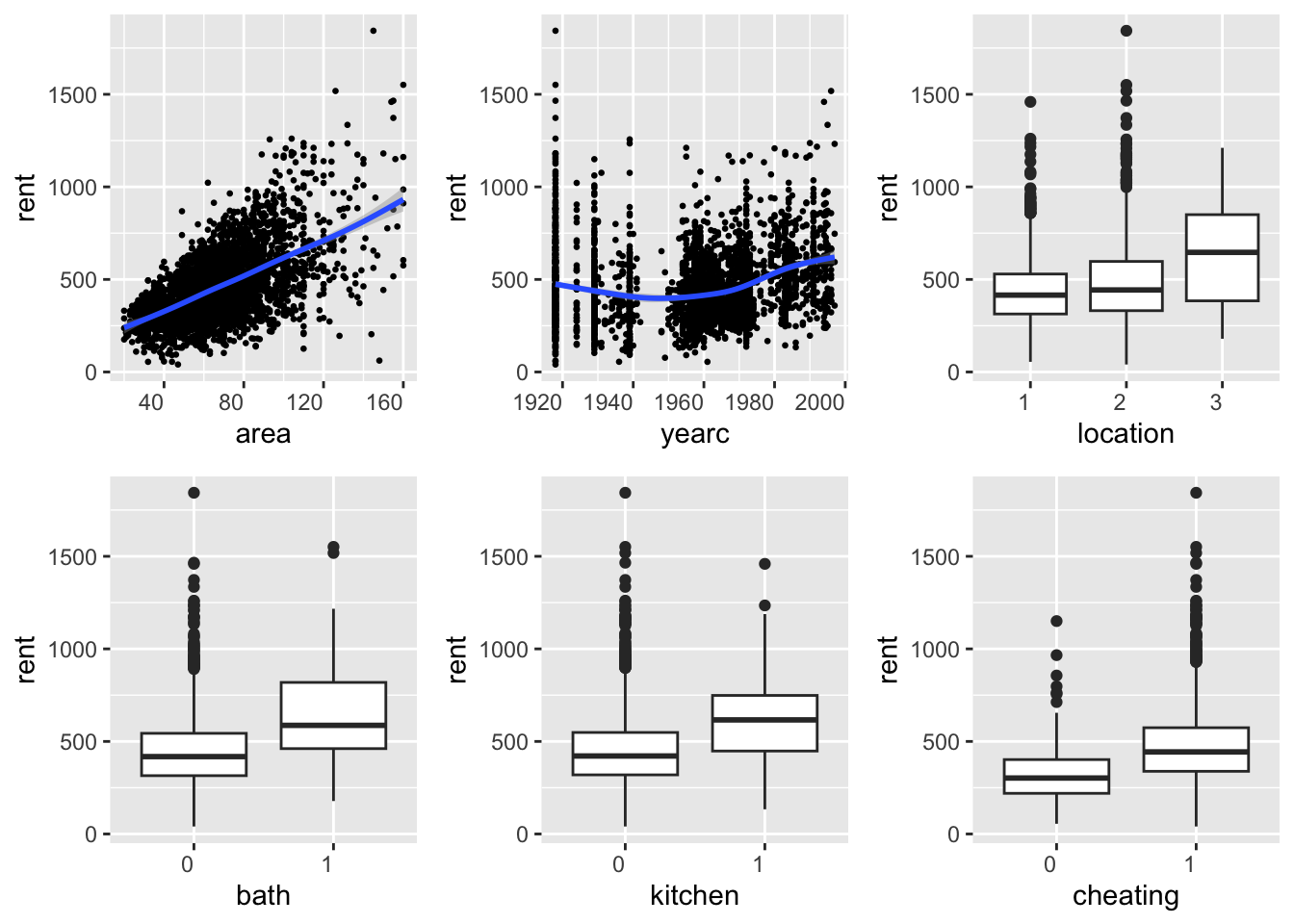
The functions data_xyplot() plots the response variable against each of the independent explanatory variables. It plots the continuous against continuous as scatter plots and continuous variables against categorical as box plot.
Note
At the moment there is no provision for categorical response variables.
da |>data_xyplot(response=rent )
 100 % of data are saved,
that is, 3082 observations.
`geom_smooth()` using method = 'gam' and formula = 'y ~ s(x, bs = "cs")'
`geom_smooth()` using method = 'gam' and formula = 'y ~ s(x, bs = "cs")'
The output of the function saves the ggplot2 figures.
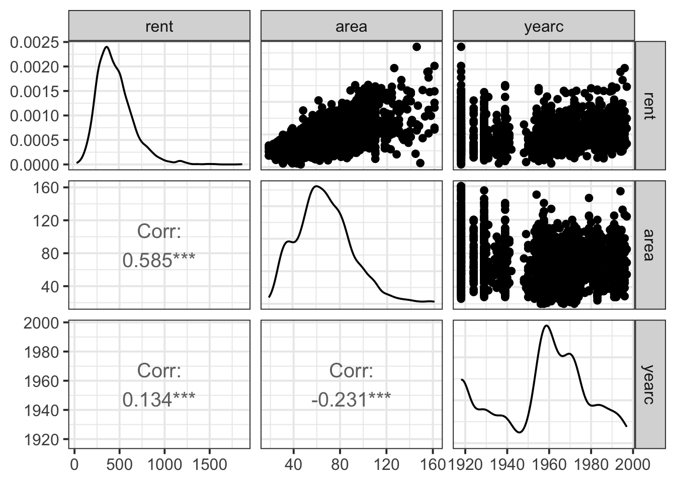
Note hat the package gamlss.prepdata do not provides pairwise plot of the explanatory variables themself but the package GGally does. here is an example ;
library(GGally)
Registered S3 method overwritten by 'GGally':
  method from
  +.gg   ggplot2
dac <- gamlss.prepdata:::data_only_continuous(da) ggpairs(dac, lower=list(continuous ="cor",combo ="box_no_facet", discrete ="count", na ="na"),upper=list(continuous ="points", combo ="box_no_facet", discrete ="count", na ="na")) +theme_bw(base_size =15)
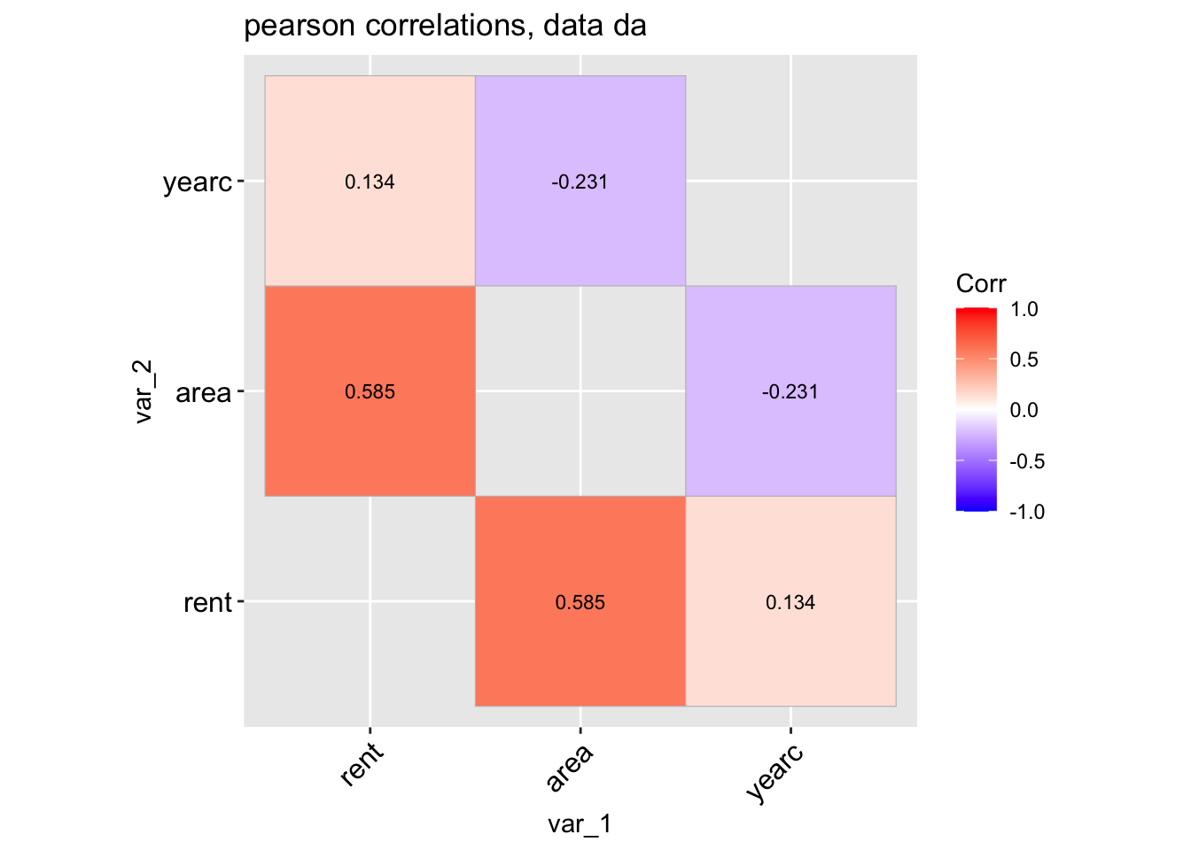
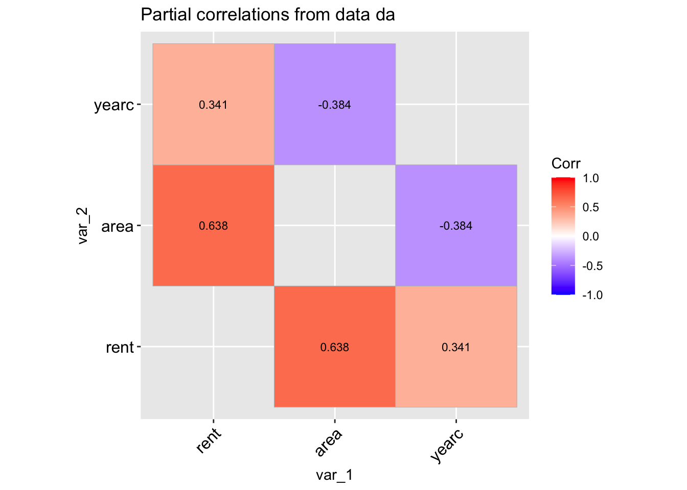
The function data_corr() is taking a data.frame object and plot the correlation coefficients of all its continuous variables.
data_cor(da, lab=TRUE)
 100 % of data are saved,
that is, 3082 observations.
4 factors have been omited from the data
Warning in data_cor(da, lab = TRUE):
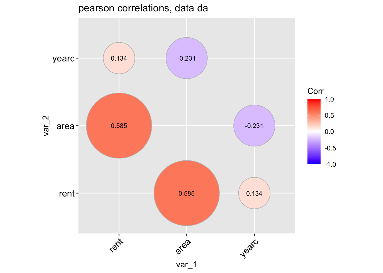
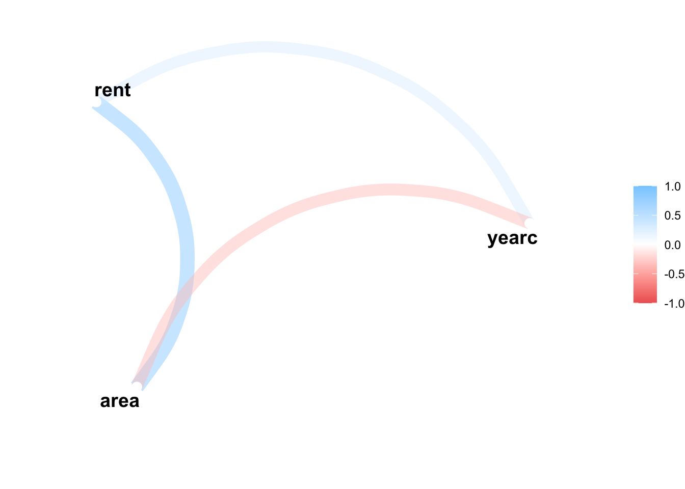
A different type of plot can be produce if we use;
data_cor(da, method="circle", circle.size =40)
 100 % of data are saved,
that is, 3082 observations.
4 factors have been omited from the data
Warning in data_cor(da, method = "circle", circle.size = 40):
To get the variables with higher, say, than $0.4 $ correlation values use;
Tabcor <-data_cor(da, plot=FALSE)
 100 % of data are saved,
that is, 3082 observations.
4 factors have been omited from the data
Warning in data_cor(da, plot = FALSE):
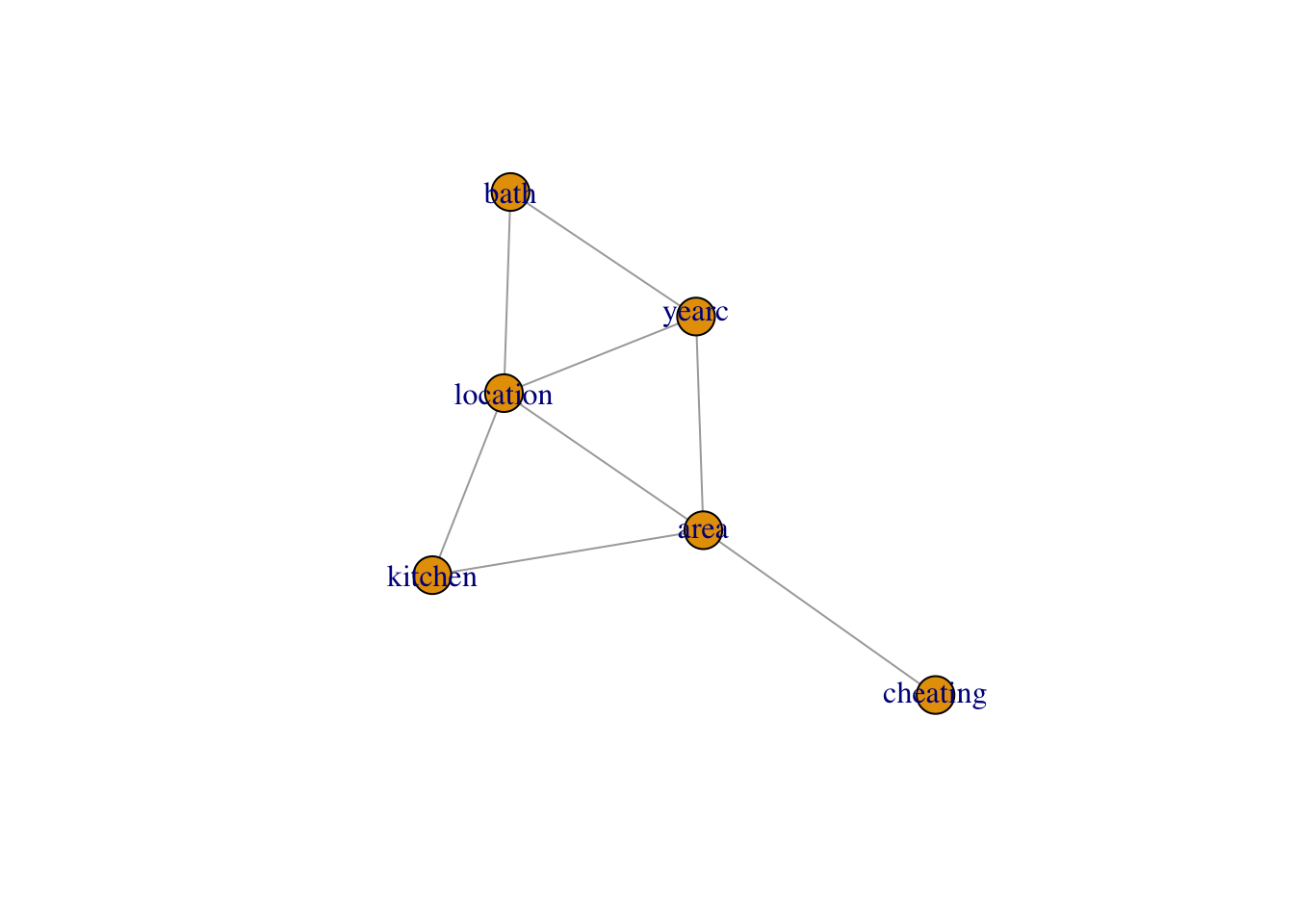
high_val(Tabcor, val=0.4)
     name1  name2  corrs
[1,] "rent" "area" "0.585"
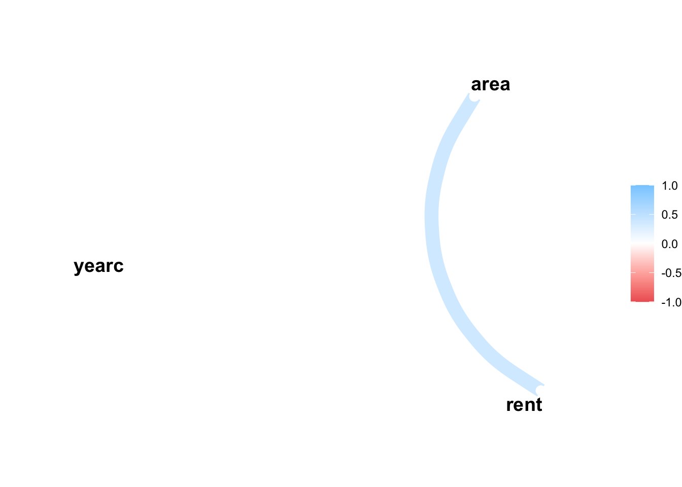
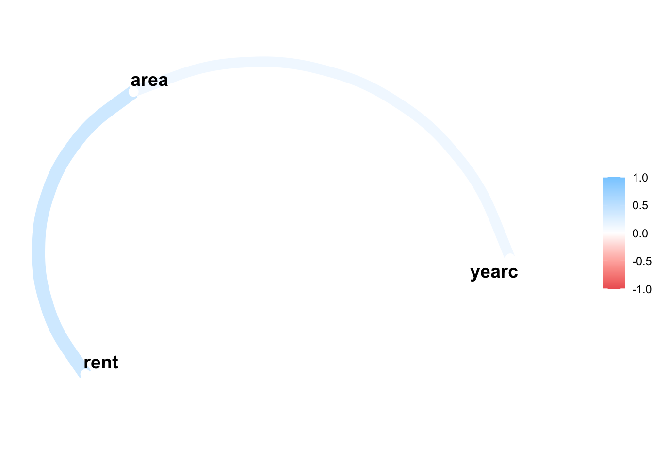
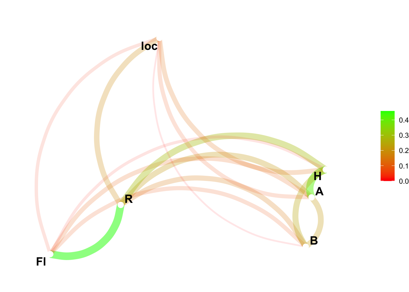
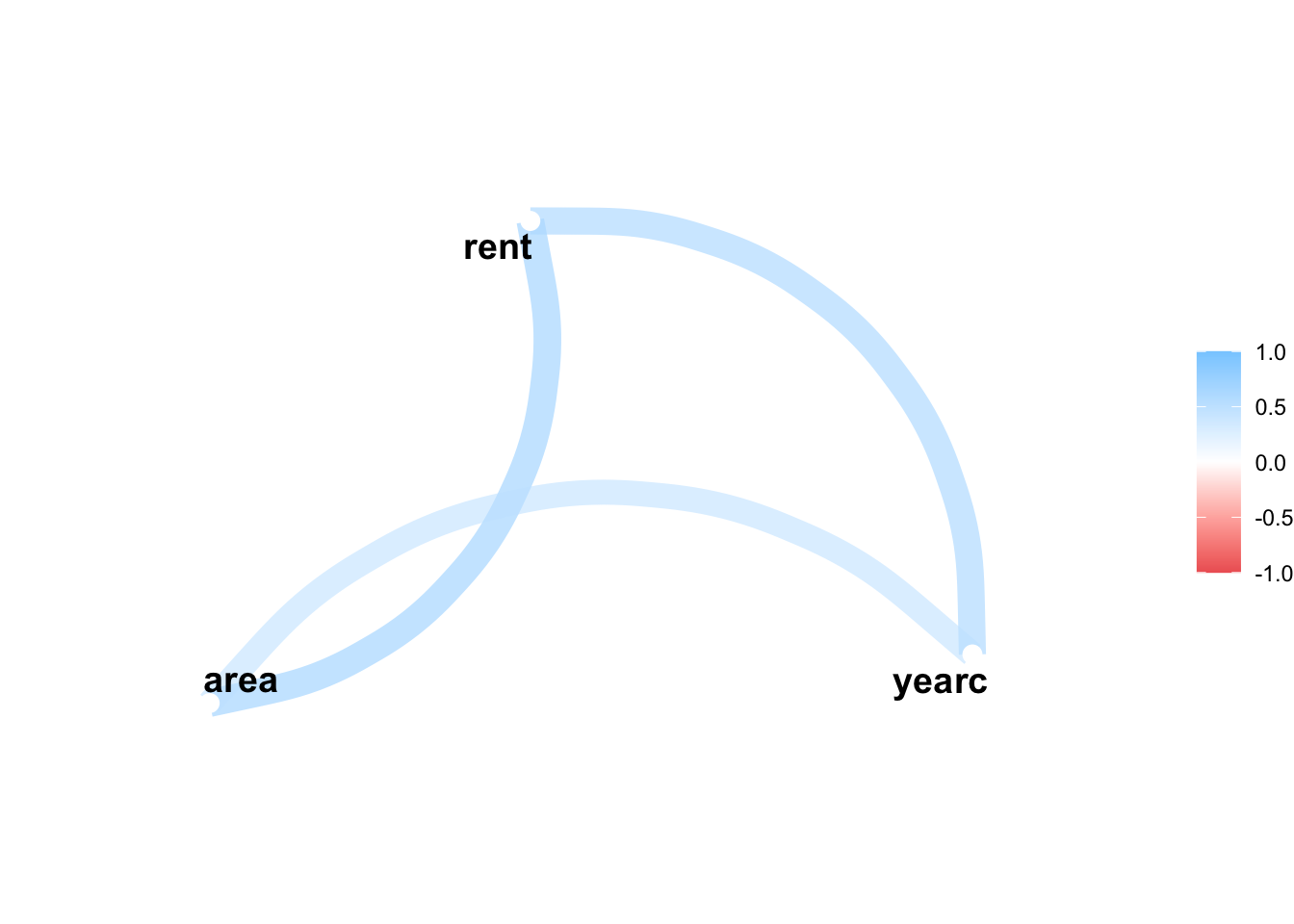
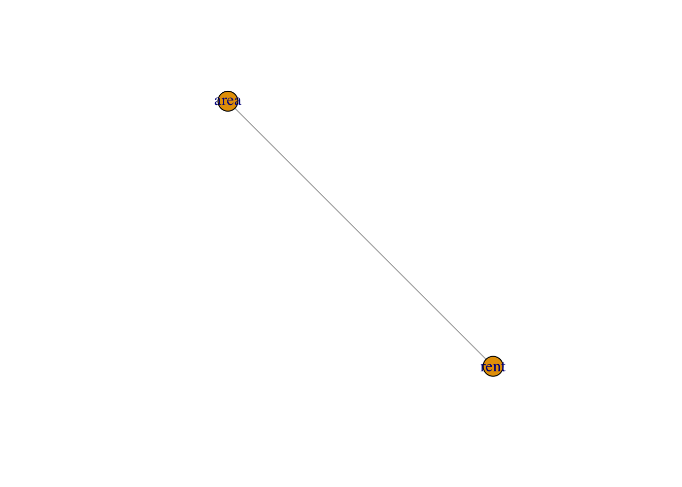
We can plot the path of those variables using the package corr;
library(corrr)network_plot(Tabcor)
Warning: Using `size` aesthetic for lines was deprecated in ggplot2 3.4.0.
ℹ Please use `linewidth` instead.
ℹ The deprecated feature was likely used in the corrr package.
  Please report the issue at <https://github.com/tidymodels/corrr/issues>.
Note that there are two functions associated with the data_cor()
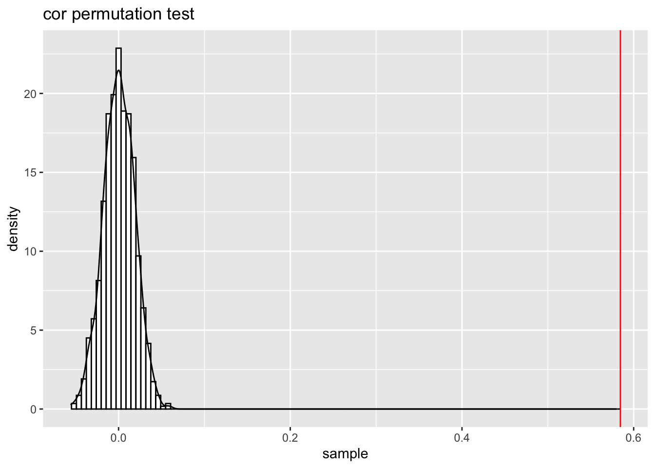
cor_perm_test(); this function test the null hypothesis that the correlation coefficients of two continuous variables is zero or not
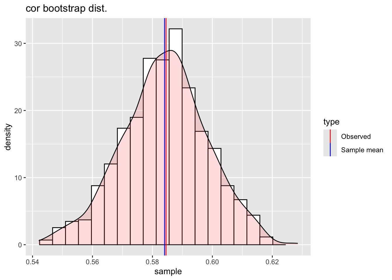
cor_boot() this function find the bootstrap distribution of the correlation coefficients of two continuous variables. This bootstrap distribution can be used then to test the probability that the correlation coefficients could be zero.
correlation between da$area and da$rent
observed: 0.591
sample mean: 0.593
bias: -0.00246
sample SD: 0.0134
sample size: 1000
plot(bb1)
Warning: Removed 2 rows containing missing values or values outside the scale range
(`geom_bar()`).
Note that the plot has the original value of the correlation marked as Observed in a red vertical line and the average of the bootstrap simulations marked as Sample mran in a blue vertical line. The difference between those two values can ve consider as an estimate of the bias.
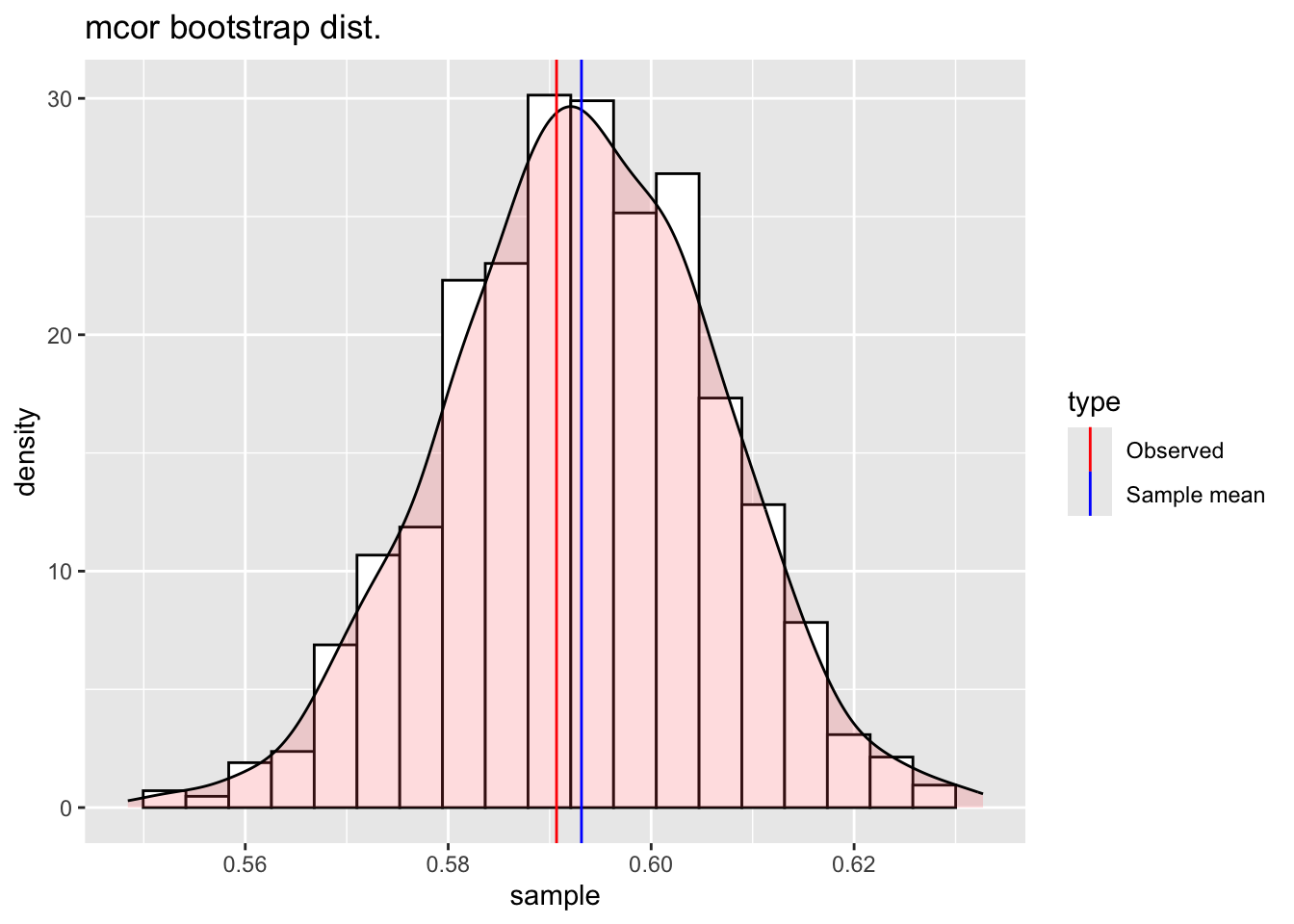
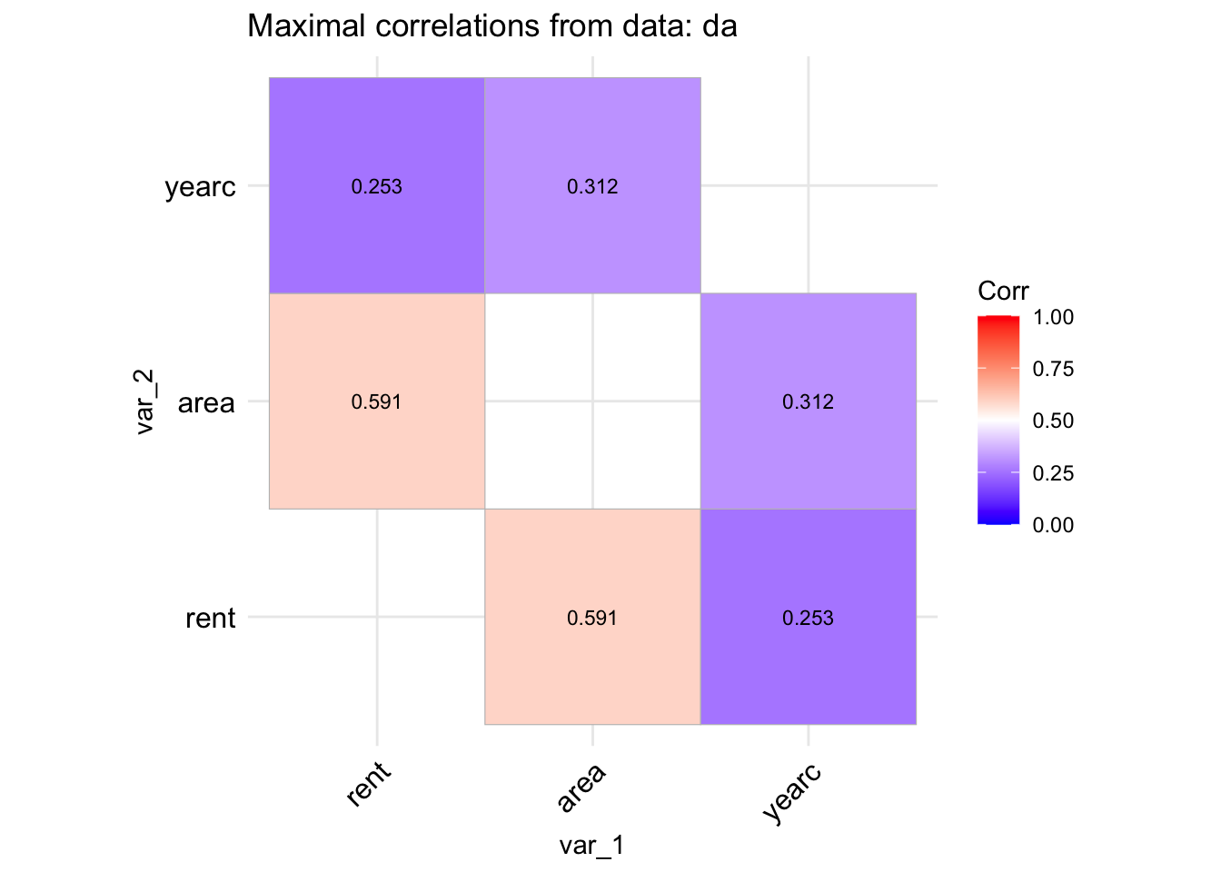
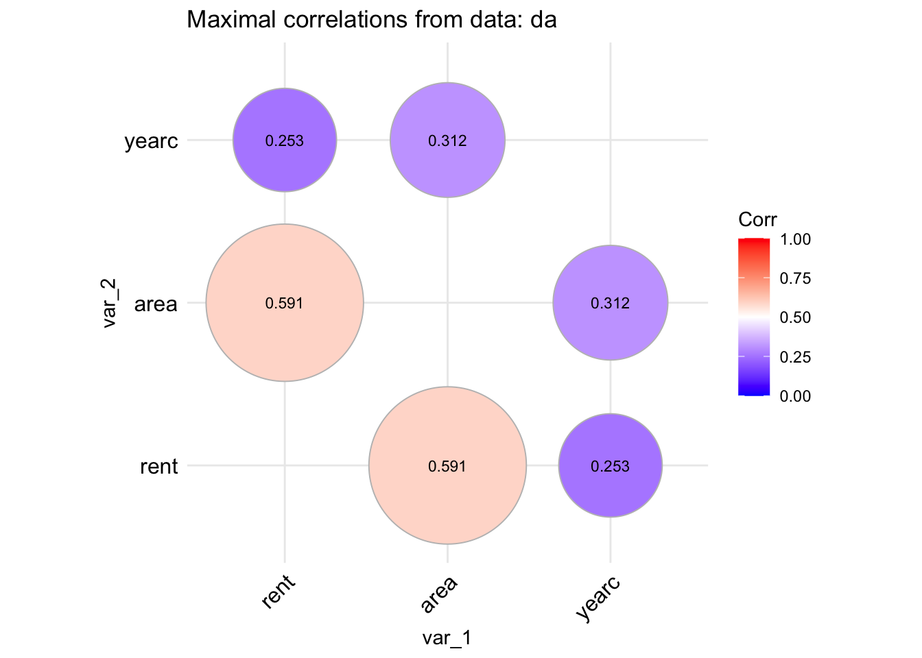
data_mcor()
The function data_mcor() is taking a data.frame object and plot the maximal correlation (non-linear) coefficients of all its continuous variables.
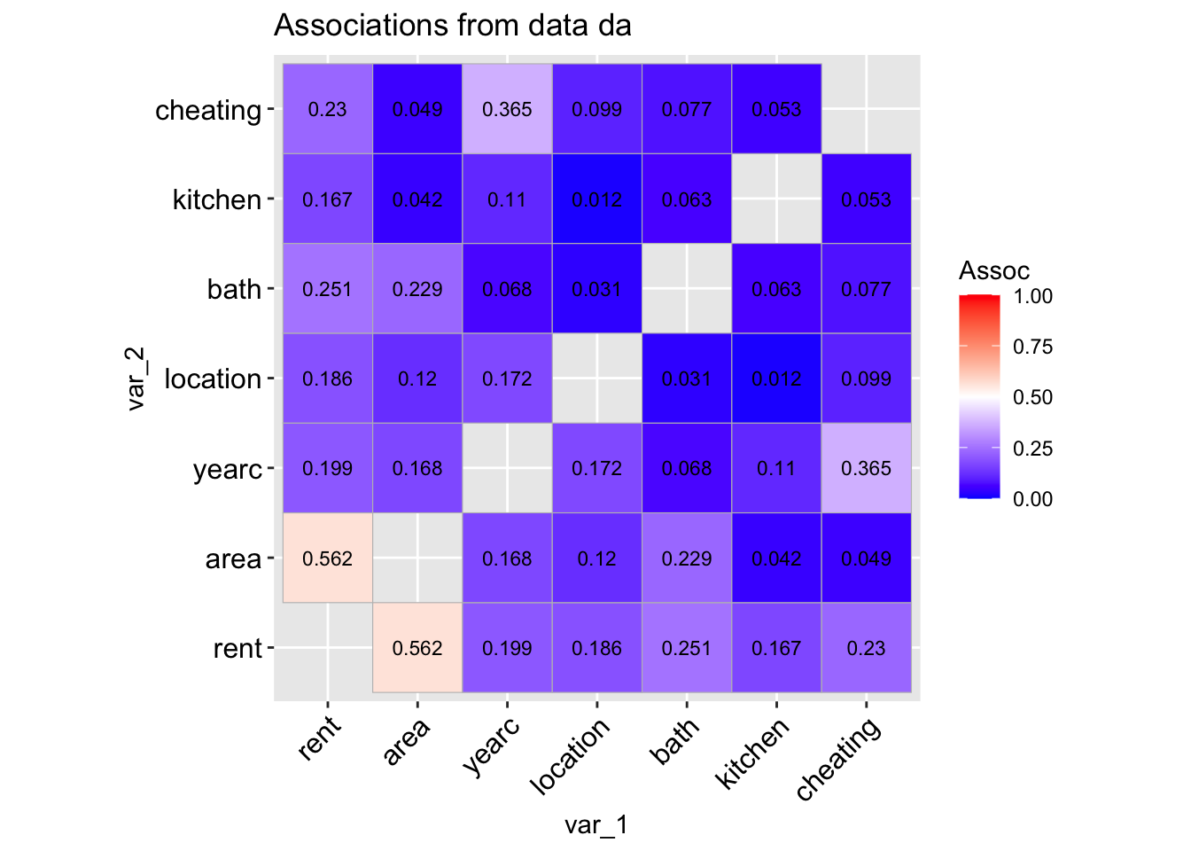
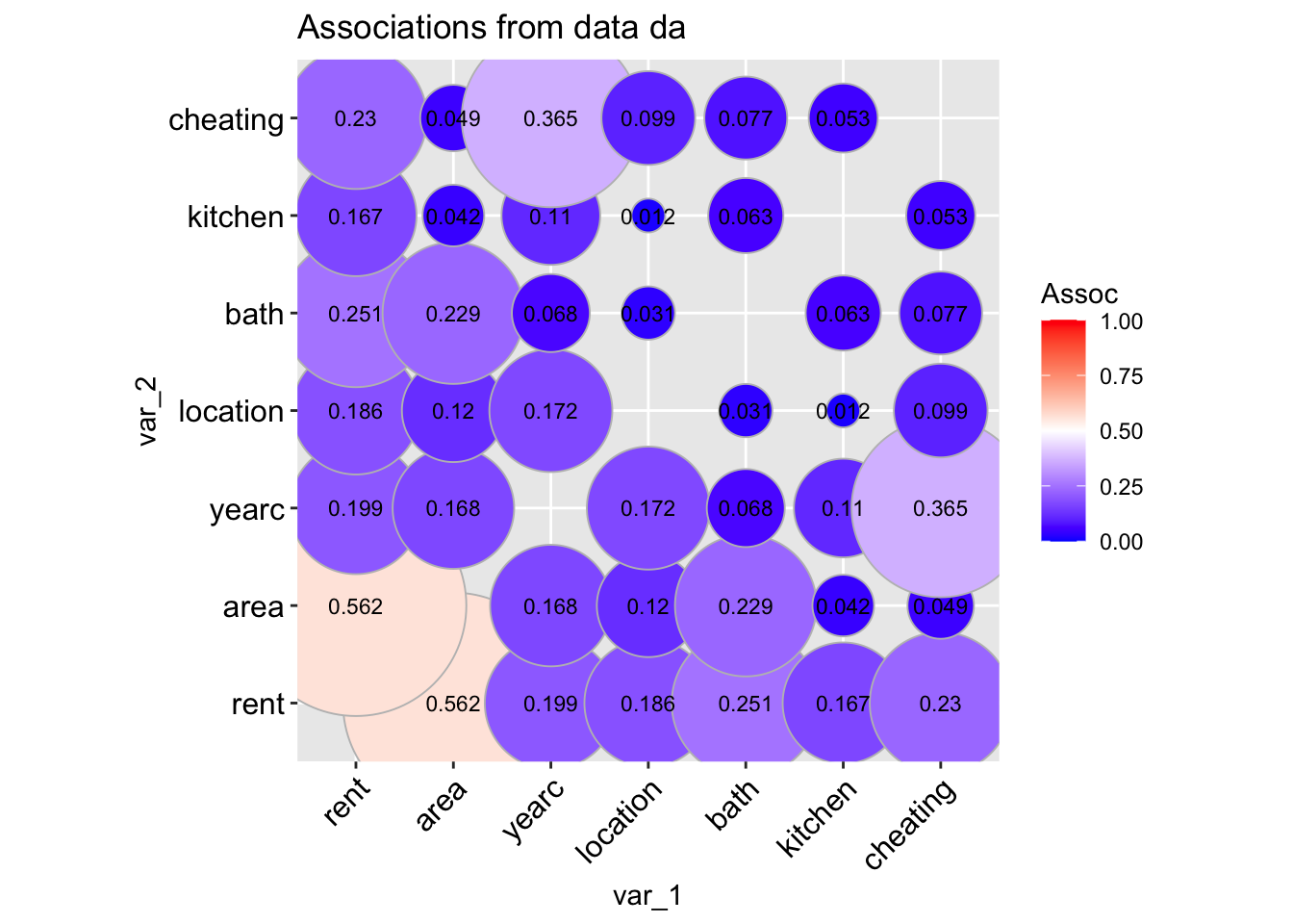
The function data_association() is taking a data.frame object and plot the pair-wise association of all its variables. The pair-wise association for two continuous variables is given by default by the absolute value of the Spearman’s correlation coefficient. For two categorical variables by the (adjusted for bias) Cramers’ v-coefficient. For a continuous against a categorical variables by the \(\sqrt R^2\) obtained by regressing the continuous variable against the categorical variable.
data_association(da, lab=TRUE)
 100 % of data are saved,
that is, 3082 observations.
A different type of plot can be produce if we use;
This function is new. Its theoretical foundation are not proven yet. The function needs testing and therefore it should be used with causion.
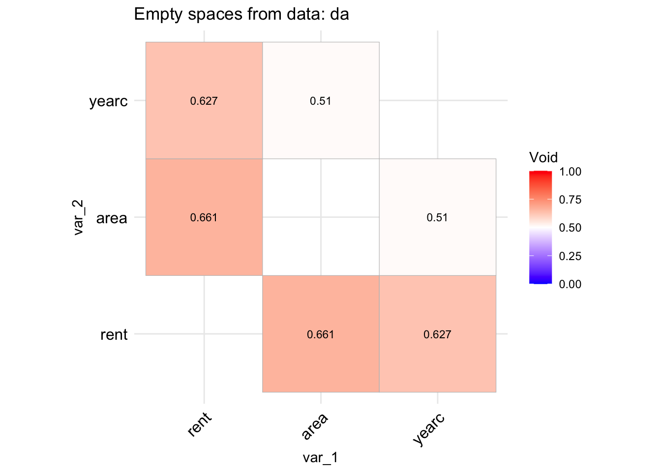
The idea behind the functions void() and its equivalent data.frame version data_void() is to be able to identify whether the data in the direction of two continuous variables say \(x_i\) and \(x_j\) have a lot of empty spaces. The reason is that empty spaces effect prediction since interpolation at empty spaces is dengerous. The function data_void() is taking a data.frame object and plot the percentage of empty spaces for all pair-wise continuous variables. The function used the foreach() function of the package foreach to allow parallel processing.
registerDoParallel(cores =9)data_void(da)
 100 % of data are saved,
that is, 3082 observations.
4 factors have been omited from the data
Warning in data_void(da):
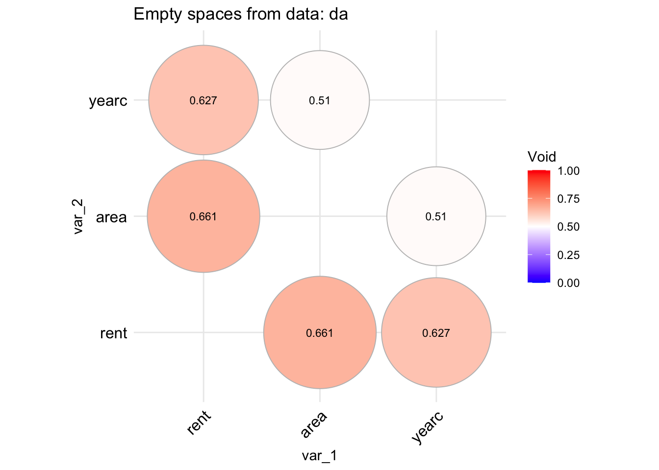
A different type of plot can be produce if we use;
data_void(da, method="circle", circle.size =40)
 100 % of data are saved,
that is, 3082 observations.
4 factors have been omited from the data
Warning in data_void(da, method = "circle", circle.size = 40):
stopImplicitCluster()
To get the variables with highter than $0.4 $ values use;
Tabvoid <-data_void(da, plot=FALSE)
 100 % of data are saved,
that is, 3082 observations.
4 factors have been omited from the data
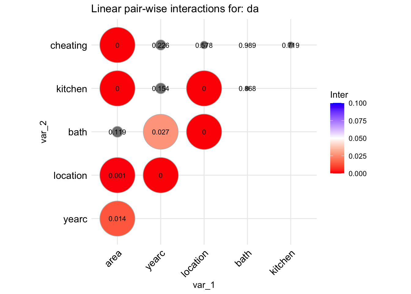
The function data_inter() takes a data.frame, fits all pair-wise interactions of the explanatory variables against the response (using a normal model) and produce a graph displaying their significance levels. The idea behind this is to identify possible first order interactions at an early stage of the analysis.
da |> gamlss.prepdata:::data_inter(response= rent)
 100 % of data are saved,
that is, 3082 observations.
 100 % of data are saved,
that is, 3082 observations.
tinter
         area yearc location  bath kitchen cheating
area       NA 0.014    0.001 0.119   0.000    0.000
yearc      NA    NA    0.000 0.027   0.154    0.226
location   NA    NA       NA 0.000   0.000    0.578
bath       NA    NA       NA    NA   0.868    0.989
kitchen    NA    NA       NA    NA      NA    0.719
cheating   NA    NA       NA    NA      NA       NA
To get the variables with lower than $0.05 $ significant interactions use;
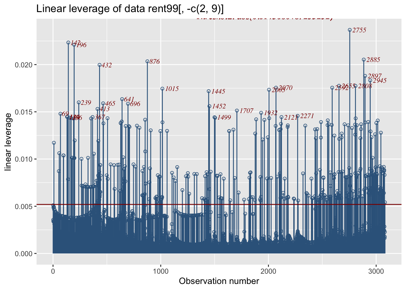
The function data_leverage() uses the linear model methodology to identify posible unusual observations within all the explanatory variables taken as a group (not individually). It fit a linear (normal) model with response, the response of the data, and all explanatory variables in the data, as x’s. It then calculates the leverage points and plots them. A leverage is a number between zero and 1. Large leverage correspond to more extremes observations for all x’s.
rent99[, -c(2,9)] |>data_leverage( response=rent)
 100 % of data are saved,
that is, 3082 observations.
Note
The horizontal line is the plot is at point \(2 \times (r/n)\), which is the threshold suggested in the literature; values beyond this point could be identified as extremes. It looks that the point \(2 \times (r/n)\) is too low (at least for our data). Instead the plot identify only observation which are in the one per cent upper quantile. That is a quantile value of the leverage at value 0.99.
Section 6.1.7 show how the information of the function data_leverage() can be combined with the information given by data_outliers() in order to confirm hight outliers in the data.
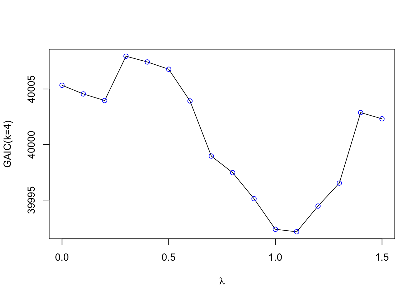
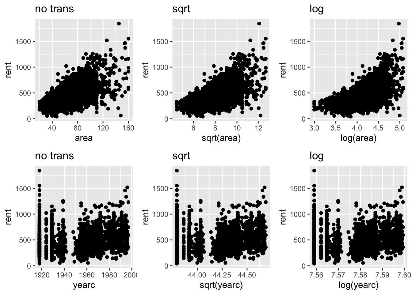
The essence of this plot is to visually decide whether certain values of \(\lambda\) in a power transformation are appropriate or not. Section 6.4 describes the power transformation, \(T=X^\lambda\) for \(\lambda>0\), in more details. For each continuous explanatory variable \(X\), the function show the response against \(X\), (\(\lambda=1\)), the response against the square root of \(X\), (\(\lambda=1/2\)) and the response against the log of \(X\) (\(\lambda \rightarrow 0\)). The user then can decide whether any of those transformation are appropriate. Note that the square root and log transformations are appropriate for righ skew variables.
gamlss.prepdata:::data_Ptrans_plot(da, rent)
 100 % of data are saved,
that is, 3082 observations.
It look that no transformation is needed for the continuous explanatory variables area of yearc.
identify outliers (using z-scores) by fitting several times the chossen family eliminating each time observations identifyied as outliers in the prievious fits
Outliers in the response variable, within a distributional regression framework like GAMLSS, are better handled by selecting an appropriate distribution for the response. For example, an outlier under the assumption of a normal distribution for the response may no longer be considered an outlier if a distribution from the t-family is assumed. Considerations of contanimnated responses data are not considered here. The function data_response(), discussed in Section 5.0.3 and uses the z-scores methodology, provides some guidelines for appropriate action to identify ouliers in the response. This section focuses on outliers in the explanatory variables.
Outliers in the continuous explanatory variables can potentially affect curve fitting, whether using linear or smooth non-parametric terms. In such cases, removing outliers from the x-variables can make the model more robust. Outliers are observations that deviate significantly from the rest of the data, but the concept also depends on the dimension being considered. An single observation value might be an outlier on an explanatory variable. A pair of observations could be an outlier when examined within a pair-wise relationships. Extreme observations identification on continuous variables, is based on how far the observation lies from the majority of the data. Pairwise plots of continuous variables could identify outliers in the two-dimensions. Leverage points are useful to identify outliers in \(r\) dimensions where \(r\) is the size of the explanatory variables.
Note
At this preliminary stage of the analysis (no model has been fitted yet), it is difficult to identify outliers among factors. This is because outliers in factors typically do not appear unusual unless are examined in combination with rest of factors or variables. Identifying factor outliers is a task better suited for the modelling stage of the analysis.
The function y_outliers() in Section 6.1.1, is applied to continuous variables only, and it uses two different methodologies (option type);
the z-scores, type="zscorses" (the default) and
the quantile rule, type="quantile".
Both methodologies are trying to remove extreme skewness in the variables before looking for outliers by using the (internal) function y_Ptrans(). The function is applied to any variable with positive values. The assumption, is that positive variables are more likely to be right skewed and therefor a power transformation will correct that. The function y_Ptrans() attempts to find the power \(\lambda\), of a transformation \(T = X^\lambda\), that minimizes the Jarque-Bera test statistic—a measure of deviation from normality. The Jarque-Bera test statistic is always non-negative and a value way from zero indicates strong evidence against normality. The goal of this methodology is to reduce extreme skewness in the data before attempt to identify the outliers. If the data are not so skewed the power transformation will genraly do no harm.
Note
At the momment we allow the power parameter of the tranformation \(\lambda\) to vary at the range \(0\) to \(1.5\). This range cover only right skewed behaviour. More work has to be done to establishes suitable range.
Now given that the positive variables are transformed (using the power transformation) and that all the rest of variables, containg negative values, remain untransformed, the z-scores methodology fits a parametertic distribution to the variable and computes the residuals of the fitted model (z-scores). The default distribution is the four parameter SHASHo distribution. The z-scores methodology identify outliers if a spesific residual (z-score) has an absolute value bigger that a predetermining value ay \(K\). The quantile rule methodology works similar. It identify an observation if it is further than \(K \times MAD\) way from the median. The value of \(K\) is set by the option value of the function y_outliers(). If the value is missing it is calculated using the formulas \(\Phi^{-1}(1/(10 \times N))\), where N is the number of observations. The two methodologies are appropriate for identifying outliers in one dimension. To identify outliers in \(p\) dimensions the function data_leverage(), see Section 6.1.7, shouls be used.
Note
Several of the graphical functions described in Section 5 are good for identify outliers visually. In fact we recommend that the function data_outliers() and its related function data_outliers_both(), data_outliers_by() and data_outliers_z() should be used in combination with functions like data_plot() or data_zscores() or y_dots() of the package gamlss.gplots.
y_outliers()
The function y_outliers() identify outliers in one \(x\) variable using the two methodologies described above, The
zscores: wherte a distribution is fitted to the data (default SHASHo), the residuals (z-scores) are taken and observations with large residuals are identified as outliers.
quantile: This is more realing with the classical methodology based on sample quantiles. An observation is identified if it far from the median. How far usually is taken as \(K\) time the Mean Absolute Deviation (MAD).
Hewe is an example using the zscores;
y_outliers(da$rent)
the x was tansformed using the power 0.2412793
named integer(0)
and here using the quantile;
y_outliers(da$rent, type="quantile")
the x was tansformed using the power 0.2412793
[1] 38 426
Note that the function y_outliers() is used by data_outliers() to identify outliers in all continuous variables in the data. There are several variation of the basic function y_outliers() described next.
The function y_outliers_both() uses both zscores and quantile methodology and reports the observations appearing in the intersection of both sets, method=intersection (the default), or the union of both, method=union.
y_outliers_both(da$rent, method="union")
the x was tansformed using the power 0.2412793
the x was tansformed using the power 0.2412793
The function y_outliers_by() splits the data according to given factor, option by before it performes the detection of outliers. It is useful if the given factor split the data in a meaningful way. Continuous variable can be split in advange to create a factors using the R function cut().
The function y_outliers_loop() tries to identify more data than the y_outliers() function by using the folwing extra loop; It starts by fitting the distribution to the data which help to identify from the z-scores certain obsevations as outliers. Thaose outliers are `then removed and the procees starts again. It stops whete there are no more observations removed. This loop allows more obsrvations to be identify and it is design to help when banch of data points masks other point to be identified as outliers.
The function y_outliers_z() tries to put the functions y_outliers_loop() and y_outliers_by() together. It works only for the z-scores methodology but its option allow different combinations of the algorithm. For example the options;
by: allows to fit for levels of a factor;
value: allows different values in th edetection of z-scores outliers;
family; allows different families of distribution to be fitted (instead of the SHASHo)
transform allows to switch off the transformation option
loop; allows looping the algorithm, TRUE or FALSE.
The function data_outliers() uses the z-scores technique described above in order to detect outliers in the continuous variables in the data. It fits a SHASHo distribution to the continuous variable in the data and uses the z-scores (quantile residuals) to identify (one dimension) outliers for those continuous variables.
data_outliers(da)
the x was tansformed using the power 0.2412793
the x was tansformed using the power 0.3872234
the x was tansformed using the power 1.499942
$rent
named integer(0)
$area
named integer(0)
$yearc
named integer(0)
As it happen no individual variable outliers were highlighted in the rent data using the z-scores methodology. In general we recommend the function data_outliers() to be used in combination of the graphical functions data_plot() and data_zscores()
The function data_leverage(), fisrt describe in Section 5.0.14, can be used to detect extremes in the continuous variables in the data by fiting a linear model with all the continuous variables in the data and then useing the higher leverage points to identify (multi-dimension) outliers for the observations for all continuous variables. By default, it identifies one percent of the observations with high leverage in the data. Here we use the function as a way to identify the obsrvation (not plottoing).
data_leverage(da, response=rent, plot=FALSE)
 100 % of data are saved,
that is, 3082 observations.
The functiondata_leverage() always identifies the top one percent of observations with the highest leverage, which may or may not be outliers. These high-leverage points can have a strong influence on model estimates. To better assess their impact, the list of high-leverage observations returned by data_leverage() should be compared with the list of outliers identified by the data_outliers() function. Observations that appear in both lists are particularly noteworthy, as they may be influential outliers that warrant further investigation.
Next we are trying the process of identifying if data with high leverage are also coincide with outliers identified using the function data_outliers() function. The function intersect() will flash out the intersection of the two set of observations. First use data_outliers()
ul <-unlist(data_outliers(da))
the x was tansformed using the power 0.2412793
the x was tansformed using the power 0.3872234
the x was tansformed using the power 1.499942
then data_leverage();
ll<-data_leverage(da, response=rent, plot=FALSE)
 100 % of data are saved,
that is, 3082 observations.
and finally we inspect the intersection of the two sets using intersect();
intersect(ll,ul)
integer(0)
Here we have zero outliers but in general we would expect to find common observations for further checking.
The idea here is to identify variables with high correlation or association with the possibility to eliminated them from the data. The first function is appropriate for continuous variables while the second for both continuous and factors. Note that the method used to identify the variables is identical to the method used in the package caret see page 5 of Kuhn and Max (2008).
data_index_cor()
The function data_index_cor(), It takes a data.frame as input calculates correlation coefficients of the continuous variables in the data and creates an index for variables which could be possible to eliminate from the further analysis.
gamlss.prepdata:::data_index_cor(rent99[,-1])
4 factors have been omited from the data
Warning in data_cor(data, type = type, plot = FALSE, percentage = percentage, :
The function data_index_association(), It takes a data.frame as input calculates the association coefficients of all the variables in the data and creates an index for variables which could be possible to eliminate from the further analysis.
Scaling is another form of transformation for the continuous explanatory variables in the data which brings the explanatory variables in the same scale. It is a form of standardization. Standardization means bringing all continuous explanatory variables to similar range of values. For some machine learning techniques, i.e., principal component regression or neural networks standardization is mandatory in other like LASSO is recommended. There are two types of standardisation
scaling to normality and
scaling to a range from zero to one.
Scaling to normality it means that the variable should have a mean zero and a standard deviation one. Note that, this is equivalent of fitting a Normal distribution to the variables and then taking the z-scores (residuals) of the fit as the transformed variable. The problem with this type of scaling is that skewness and kurtosis in the standardised data persist. One could go further and fit a four parameter distribution instead of a normal where the two extra parameters could account for skewness and kurtosis. The function data_scale() described in Section 6.3.1 it gives this option with te argument family in which can used to specify a different distribution.
data_scale()
The function data_scale() perform scaling to all continuous variables an a data set. Note that factors in the data set are left untouched because when fitted within a model they will be transform to dummy variable which take values 0 or 1 (a kind of standardization). The response is left also untouched because it is assumed that an appropriate distribution will be fitted. The response variable has to be declared using the argument response. First we use data_scale() to scale to normality.
head(data_scale(da, response=rent))
area yearc location bath kitchen cheating
132 68 3 2 2 2
 100 % of data are saved,
that is, 3082 observations.
As we mention before scaling to normality is equivalent of fitting a Normal variable first. The problem with scaling to normality is that if the variables are highly skew or kurtotic scaling them to normality does correct for skewness or kurtosis. Using a parametric distribution with four parameters some of which are skewness and kurtosis parameters it may correct that. Next we standardised using the SHASHo distribution;
In the context of outliers, the focus on how far a single observation deviates from the rest of the data. However, when considering transformations, the goal shifts toward a better capturing of the relationship between a continuous predictor and the response variable. Specifically, we aim to model peaks and troughs in the relationship between a single x-variable and the response better. To achieve this, it is sometimes sufficient to stretch the x-axis so that the predictor variable is more evenly distributed within its its range. A common approach for this is to use a power transformation of the form \(T = X^\lambda\). This transoformation can reduce the curvature in the response and make the curve fitting easier. Importantly, the power transformation smoothly transitions into a logarithmic transformation as \(\lambda \to 0\), since: \(\frac{X^{\lambda} - 1} {\lambda} \rightarrow \log(X) \quad \text{as } \lambda \to 0\). Thus, in the limit as \(\lambda \to 0\) is the power transformation is the log transformation \(T = \log(X)\).
Note
The power transformation is a subclass of the shifted power transformation \(T = (\alpha + X)^\lambda\) which is not consider here
The aim of the power transformation is to make the model fitting process more robust and reliable and maximizing the information extracted from the data. There are three different functions in gamlss.prepdata dealling with power transformations, xy_Ptrans(), data_Ptrans() and data_Ptrans_plot()
Note
It’s important to distinguish between the concepts of transformations (the subject of this section) and of feature extraction, a term often used in machine learning. We refer to transformations as functions applied to a individual explanatory variables while we use feature extraction when multiple explanatory variables are involved. In both cases, the goal is to enhance the model capabilities.
Time series data sets consist of observations collected at consistent time intervals—e.g., daily, weekly, or monthly. These data require special treatment because observations that are closer together in time tend to be more similar, violating the usual assumption of independence between observations. A similar issue arises in spatial data sets, where observations that are geographically closer often exhibit spatial correlation, again violating independence.
Many data sets include spatial or temporal features —such as longitude and latitude or timestamps (e.g., 12/10/2012)— those variables are can be used for for modeling directly, but also for interpreting or visualization of the results. If temporal or spatial information exists in the data, it is essential to ensure these features are correctly read and interpreted in R. For instance, dates in R can be handled using the as.Date() function. To understand its functionality and options associated with the function please consult the help documentation via help("as.Date"). Below, we provide two simple functions of how to work with date-time variables.
time_dt2dh()
Suppose the variable dt contains both a date and a time. We may want to extract and separate this into two components: one containing the date, and another capturing the hour of the day.
The second example contains time given in its common format, c("12:35", "10:50") and we would like t change it to numeric which we can use in the model.
Partitioning the data is essential for comparing different models and checking for overfitting. Overfitting occurs when a model fails to generalize well to new data, typically because it is too closely fitted to the data. In contrast, underfitting refers to a poor model that fails to capture the essential patterns in both fitted and the new data, resulting to a model that is far the population intended to represent. It common to refer to data used for fitting the model as training data and the new data as test data.
Figure 1 shows different ways the data can be partitioned. A dataset can be split once, in holdout samples, or split multiple times using cross validation, CV, or bootstrap. For large datasets, it is common to split the data into a training set and two holdout samples, the test set, and, if needed the validation set. The training set is used for fitting the models, the test set is used to evaluate the prediction power and also to compare models, and the validation set is used for tuning the hyperparameters. [Note that for additive smoothing regression models, the hyper parameters are the smoothing parameters.] Observations in the training set are often referred to as the in-bag data, while observations in the test or validation set are termed the out-of-bag data.
Partitioning the data into training, test, and validation sets should be done randomly. This bring us to the two possible problems which could occurred when splitting the data; The zero variance variable and the extreme values problems. The zero variance variable (or nearly zero variance problem) occurs when a variable in the data (could be a factor) has only few distinct values and the frequency one of them is very low. For example, if we have the factor gender with mostly female values and only few male and we randomly portioning the data, there is a good change that all males could end up in only one of the partitions. That is, one of the partition would have factor gender properly with two levels, while the other partition with only one level. This would make the fitting and interpretation of the model difficult. One should check if this is the case. The extreme values problem is similar in nature but will effect overfitting. Extreme values could occurred in both the explanatory and the response variables. for the first case we have deal with outliers in Section 6.1 we concentrate here on extreme values in the response. Extreme values in the response (if they genuine) are of great importance for risk analysis. There is a danger thet such evens when splitting the data can go to one partition and not to the other. Any evaluation of risks in this case could be potentially wrong. One possible solution could be repeated partition, i.e bootstrap.
Bootstrap, middle of 1, is a repeated partition method. In the classical, non-parametric bootstrap, the index of the data i.e. \(1,2,\ldots,n\) is sampled with replacement \(B\) times and the model is refitted the on the re-sample data. In the Bayesian bootstrap the data are weighted using weighted samples from a multinomial distribution. \(B\) re-weighted models are refitted. While both classical and Bayesian bootstraps are computationally expensive, they provide additional insights into the model and in particular the variability of all of its parameters. A sample of length \(B\) is obtained for all the parameters of interest.
flowchart TB
  A[Data] --> B{Holdout}
  A --> C{K-fold-CV}
  A --> D{Bootstrap}
  B --> E[Training]
  E --> F[Validate]
  F --> G[Test]
  D --> H[Non-parametric]
  D --> K[Bayesian]
  C -->  L[LOO]
Figure 1: Different ways of splitting data to get in order to get more information”
In \(K\)-fold cross-validation, (right part of Figure 1), the data are split into \(K\) sub-samples. The model is then fitted \(K\) times, each time using \(K-1\) sub-samples for training and the remaining one sub-sample as test data set. By the end of the process, all \(n\) observations will have been used as test data exactly once. This is the main advantage of \(K\)-fold cross-validation is that provides reliable test data for model evaluation, (with the cost of fitting \(K\) models). Leave-One-Out Cross-Validation (LOO) is a special case of K-fold cross-validation, where the model is trained on \(n-1\) observations and tested on the remaining single observation, iterating this process \(n\) times. Consequently, \(n\) different models are refitted.
Note
Repeated partitions (i.e. bootstrapping and k-fold cross validation) could mitigating some of the problems associated from a single partitions.
Data partitioning help in selection of models, model diagnostics and detection of overfitting. Here are some rules of thump applied to distributional regression models;
if the residuals from the training data and the test data sets behave well, one is confidence, that the distributional assumption is adequate.
if the fitted model performs reasonably well (using a measure of goodness-of-fit) on both the training and the test data sets, one can be confident that overfitting has been avoided.
All methods in Figure 1, need performance metrics. Those metrics can help can: i) facilitate model comparison, ii) detect overfitting, and iii) select hyper-parameters.
Various goodness-of-fit measures can be used to check and compare different distributional regression models. One of the most popular methods which do not required partition of the data is the Generalized Akaike Information Criterion (GAIC), see Akaike (1983). To calculate the GAIC, only the in-bag data are required. However, calculating the GAIC requires an accurate measure of the degrees of freedom used to fit the model. For mathematical (stochastic) models, the degrees of freedom are straight forward to define as they correspond to the number of estimated parameters. In contrast, for over-parametrised algorithmic models like neural networks, estimating the degrees of freedom is challenging. Note that the degrees of freedom serve as a measure of the model’s complexity. We expect more complex models to be closer to the training data, which may reduce their ability to generalize well to new data (overfitting).
Note
Note that the most common of goodness-of-fit measures used in machine learning models requaring data partition are not appropriate for distributional regression model like GAMLSS. This because those measures concentrate in the behaviour at the centre of the distribution of the response which may or not be the focus of the study.
The most common measures of goodness-of-fit used in machine learning models with partitioning are;
RMSE: root mean squared error;
MAE: mean absolute error;
\(R^2\): and
MAPE: mean absolute percentage error.
All those measures of goodness-of-fit are OK is someone is interested how the middle part of the distribution of the response is behaving but are NOT god if the interest is in the tail or if the distribution is very skew. For distributional regression model the following are more appropriate measures of goodness-of-fits.
the log-likelihood: i.e. \(\ell=\log L\), or equivalent the deviance\(d=-2 \ell\)
CRPS; the continuous rank probability scores.
Note that in general goodness-of-fit measure could be can applied to both the in bag and out of bag data sets;
Computationally partition of the data for any distributional regression model, can be achieved in different ways;
by splitting the original data frame in different subsets;
by using a factor which classifies the partitions of data sets;
by indexing the original data, i.e. data[index,],
by using prior weights in the fitting.
So while we would like to think data partitioning as cutting of the original data into different subset (case 1 above), there is no inherent need for physically partition into the subgroups when fitting the models since the same results can be achieved with different methods. For example using prior weights in a \(K\)-fold cross-validation, we need \(K\) dummy vectors \(i_k\). The dummy vectors take the value of 1 for the \(k\)-th set of observations and \(0\) for the rest.
The function data_part() creates a factor for holdout or k-fold CV partitions. The data_part_list() creates a list with different data.frames for holdout or k-fold CV partitions. The function data_boot_index() and data_Kfold_index() creates appropriate vector for indexing, while data_boot_weights() and data_Kfold_weights() generates the appropriate vectors for prior weights.
This is not a partition funtion but randomly select a specified porpotion of the data
Here are the data partition functions.
data_part()
The function data_part() it does not partitioning the data as such but adds a factor called partition to the data indicating the partition. By default the data are partitioned into two sets the training ,train, and the test data, test.
Note, that use of the option partition has the following behaviour;
partition=2L (the default) the factor has two levels train, and test.
partition=3L the factor has three levels train, val (for validation) and test.
partition > 4L say K then the levels are 1, 2…K. The factor then can be used to identify K-fold cross validation, see also the function data_Kfols_CV().
The function data_part_list() creates a list of dataframes which can be used either for single partition or for cross validation. The argument partition allows the splitting of the data to up to 20 subsets. The default is a list of 2 with elements training and test (single partition).
Here is a single partition in train and test data sets.
allda <-data_part_list(rent) length(allda)
[1] 2
dim(allda[["train"]]) # training data
[1] 1200 9
dim(allda[["test"]]) # test data
[1] 769 9
Here is a multiple partition for cross validation.
The function data_boot_index() create two lists. The first called IB (for in-bag) and the second OOB, (out-of-bag). Each ellement of the list IB can be use to select a bootstrap sample from the original data.frame while each element of OOB can be use to select the out of sample data points. Note that each bootstap sample approximately contains 2/3 of the original data so we expact on avarage to 1/3 to be in OOB sample.
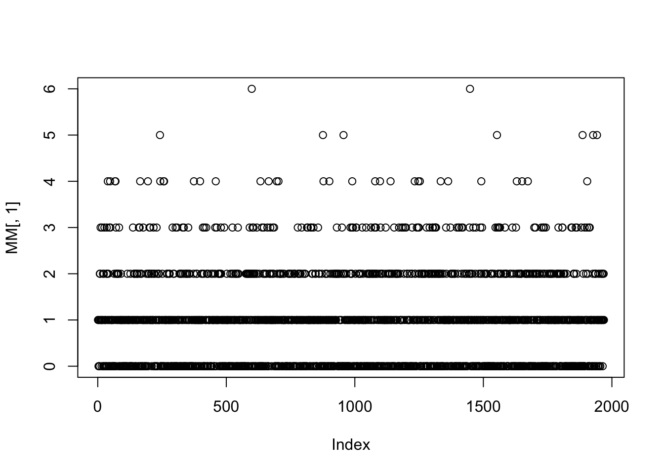
The function data_boot_weights() create a \(n \times B\). matrix with columns possible weights for bootstap fits. Note that each bootstap sample approximately contains .666 of the original obsbation so we in general we expect 0.333 of the data to have zero weights.
MM <-data_boot_weights(rent, B=10)
The M is a matrix which columns can be used as weights in bootstrap fits; Here is a plot of the first column
The function data_Kfold() creates a matrix which columns can be use for cross validation either as indices to select data for fitting or as prior weights.
The function data_Kfold() creates a matrix which columns can be use for cross validation either as indices to select data for fitting or as prior weights.
The function data_cut() is not included in the partition Section for its data partitioning properties. It is designed to select a random subset of the data specifically for plotting purposes. This is especially useful when working with large datasets, where plotting routines—such as those from the ggplot2 package—can become very slow.
The data_cut() function can either: • Automatically reduce the data size based on the total number of observations, or • Subset the data according to a user-specified percentage.
Here is an example of the function assuming that that the user requires \(50%\) of the data;
da1 <-data_cut(rent99, percentage=.5)
 50 % of data are saved,
that is, 1541 observations.
dim(rent99)
[1] 3082 9
dim(da1)
[1] 1541 9
The function data_cut() is used extensively in many plotting routines within the gamlss.ggplots package. When the percentage option is not specified, a default rule is applied to determine the proportion of the data used for plotting. This approach balances performance and visualization quality when working with large datasets.
Let \(n\) denote the total number of observations. Then:
if \(n \le 50,000\): All data are used for plotting.
if \(50,000 < n \le 100,000\): 50% of the data are used.
If \(100,000 < n \le 1,000,000\): 20% of the data are used.
If \(n>1,000,000\) : 10% of the data are used.
This default behaviour ensures that plotting remains efficient even with very large datasets.
All functions listed below belong to the gamlss.ggplots package, not the gamlss.prepdata package. However, since they can be useful during the pre-modeling stage, they are presented here. The later version of the gamlss.ggplots can be found in https://github.com/gamlss-dev/gamlss.ggplots
In the following function, no fitted model is required—only values for the parameters need to be specified.
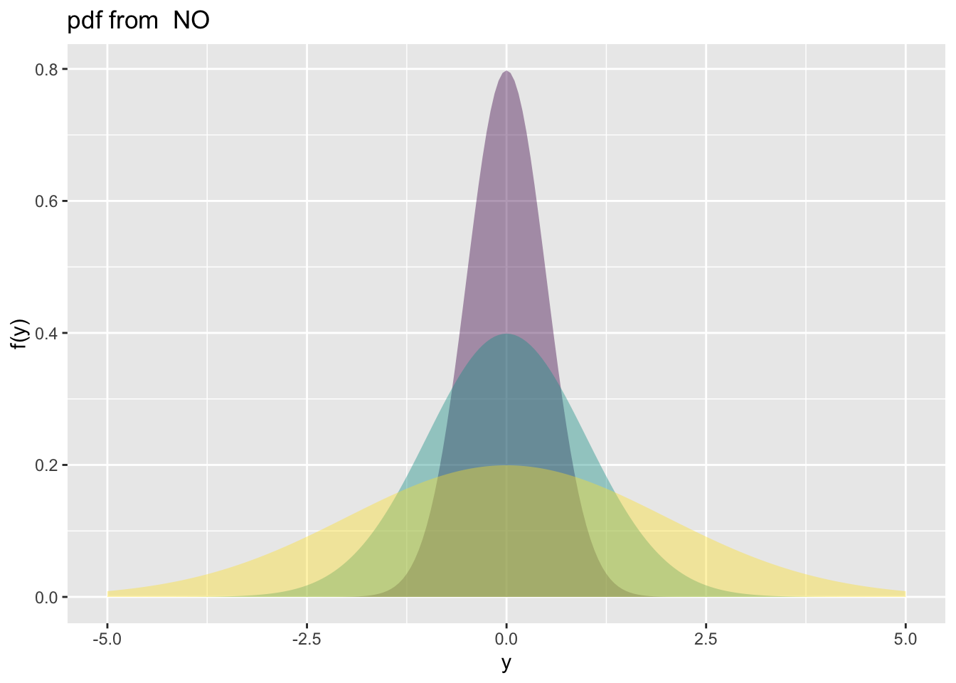
family_pdf()
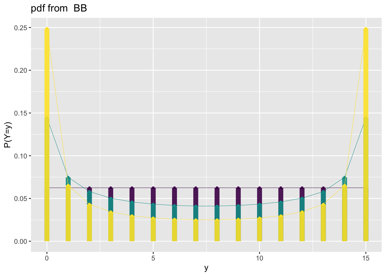
The function family_pdf() plots individual probability density functions (PDFs) from distributions in the gamlss.family package. Although it typically requires the family argument, it defaults to the Normal distribution (NO) if none is provided.
family_pdf(from=-5,to=5, mu=0, sigma=c(.5,1,2))
Figure 2: Continuous response example: plotting the pdf of a normal random variable.
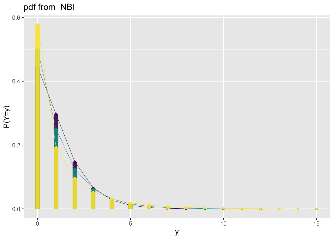
The following demonstrates how discrete distributions are displayed. We begin with a distribution that can take infinitely many count values—the Negative Binomial distribution;
Figure 4: Beta binomial response example: plotting the pdf of a beta binomial.
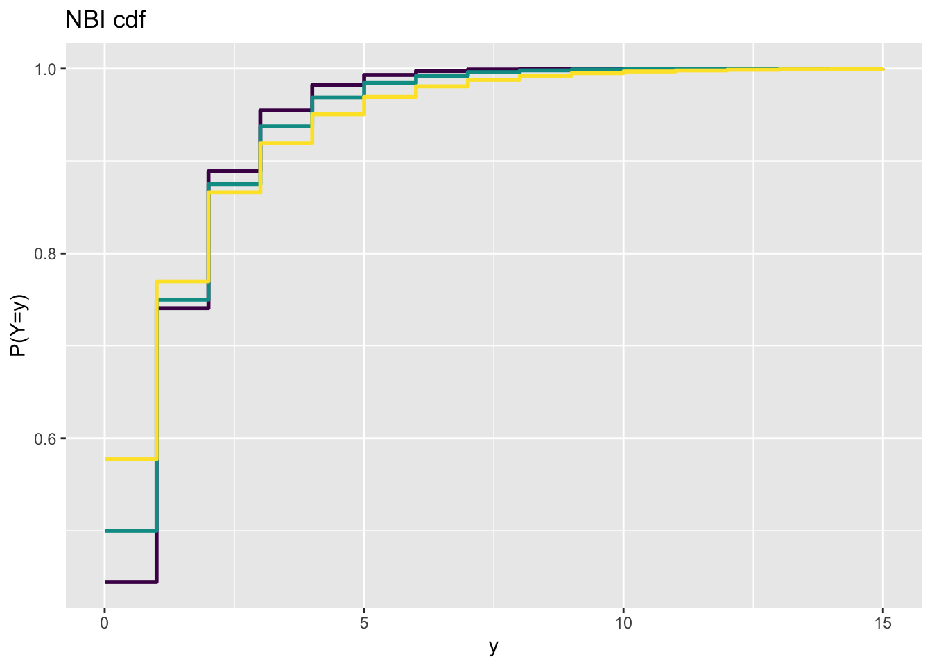
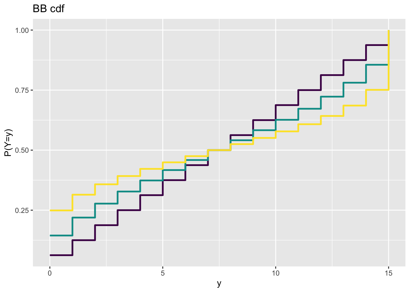
family_cdf
The function family_cdf() plots cumulative distribution functions (CDFs) from the gamlss.family distributions. The primary argument required is the family specifying the distribution to be used.
Figure 6: Count response example: plotting the cdf of a beta binomial.
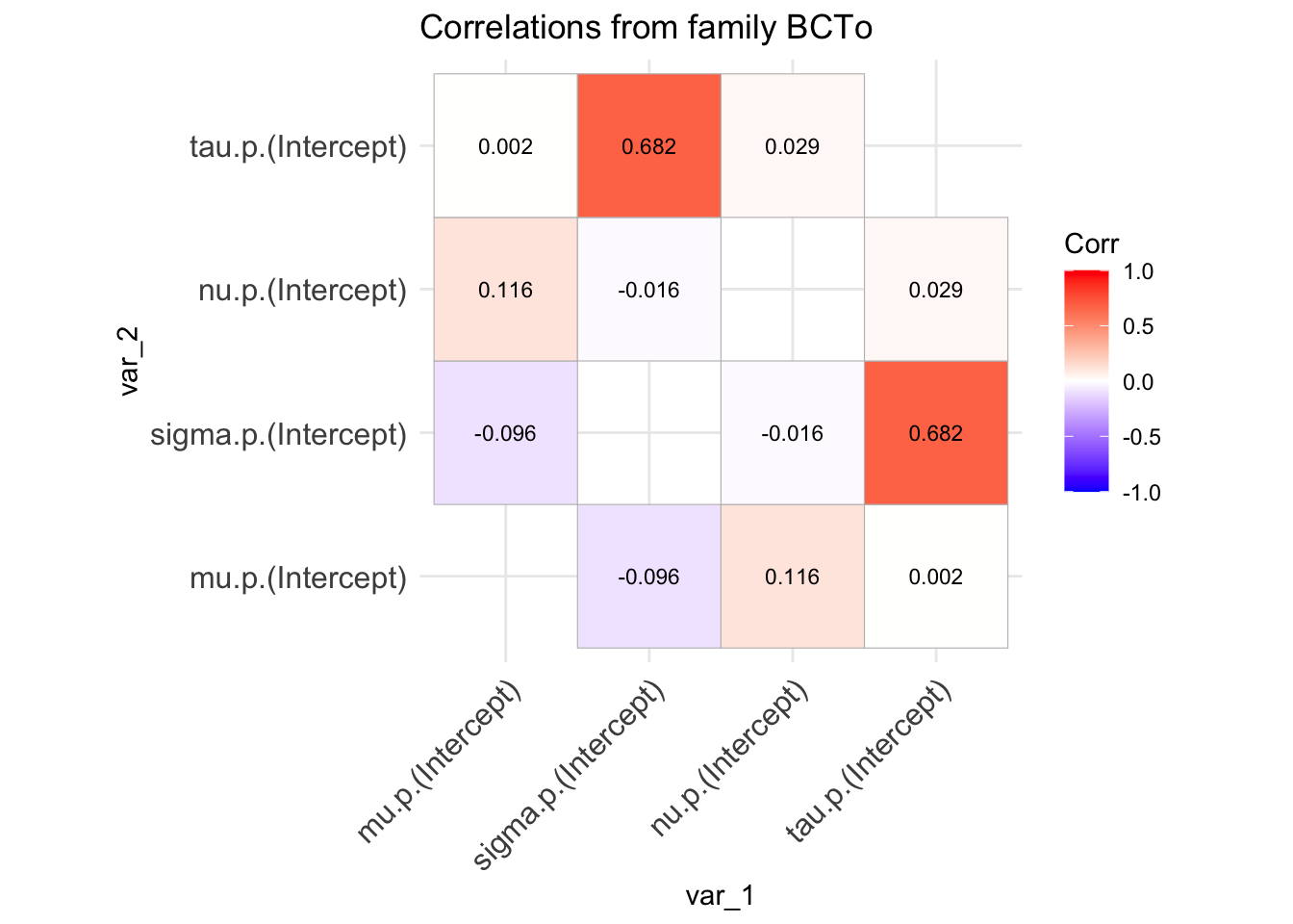
family_cor()
The function family_cor() offers a basic method for examining the inter-correlation among the parameters of any distribution from the gamlss.family. It performs the following steps:
Generates 10,000 random values from the specified distribution.
Fits the same distribution to the generated data.
Extracts and plots the correlation coefficients of the distributional parameters.
These correlation coefficients are derived from the variance-covariance matrix of the fitted model.
Warning
This method provides only a rough indication of how the parameters are correlated at specific values of the distribution’s parameters. The correlation structure may vary significantly at different points in the parameter space, as the distribution can behave quite differently depending on those values.
Figure 7: Family correlation of a BCTo distribution at specified values of the parameters.
References
Akaike, H. 1983. “Information Measures and Model Selection.”Bulletin of the International Statistical Institute 50 (1): 277–90.
Kuhn, and Max. 2008. “Building Predictive Models in r Using the Caret Package.”Journal of Statistical Software 28 (5): 1–26. https://doi.org/10.18637/jss.v028.i05.
Rigby, R. A., and D. M. Stasinopoulos. 2005. “Generalized Additive Models for Location, Scale and Shape (with Discussion).”Applied Statistics 54: 507–54.
Rigby, R. A., D. M. Stasinopoulos, G. Z. Heller, and F. De Bastiani. 2019. Distributions for Modeling Location, Scale, and Shape: Using GAMLSS in r. Boca Raton: Chapman & Hall/CRC.
Stasinopoulos, D. M., R. A. Rigby, G. Z. Heller, V. Voudouris, and F. De Bastiani. 2017. Flexible Regression and Smoothing: Using GAMLSS in r. Boca Raton: Chapman & Hall/CRC.
Stasinopoulos, M. D., T. Kneib, N. Klein, A. Mayr, and G. Z Heller. 2024. Generalized Additive Models for Location, Scale and Shape: A Distributional Regression Approach, with Applications. Vol. 56. Cambridge University Press.