Regression

Mikis Stasinopoulos

Bob Rigby

Fernanda De Bastiani

Introduction

• Regression models
• Data
• Distributions
• Fitting
• Selection
• Comparison
• Interpretation

Through a simple data example

Regression models

• Models and statistical modelling

• Assumptions

• Regression Models

• Distributional Regression

• Example

Statistical modelling

Statistical models

“all models are wrong but some are useful”.

– George Box

• Models should be parsimonious

• Models should be fit for purpose and able to answer the question at hand

• Statistical models have a stochastic component

• All models are based on assumptions.

A common theme in the following scientific subjects; statistical analysis; statistical inference; statistical modelling; machine learning; statistical learning; data mining; information harvesting; information discovery; knowledge extraction; data analytics, is data.

Assumptions

• Assumptions are made to simplify things

• Explicit assumptions

• Implicit assumptions

• it is easier to check the explicit assumptions rather the implicit ones

Model circle

flowchart TB
  A[model] --> B(assumptions) 
  B --> C[fit] --> D{check} -->|adequate| E(stop) 
  D --> |not good| B

We keep going until we find an adequate model

Regression

• \[ X \stackrel{\textit{M}(\theta)}{\longrightarrow} Y \]
• \(y\): targer, the y or the dependent variable
• \(X\): explanatory, features, x’s or independent variables or terms

\(M(\theta)\) is a model depending on parameters \(\theta\)

Linear Model

• standard way

\[ \begin{equation} y_i= b_0 + b_1 x_{1i} + b_2 x_{2i}, \ldots, b_p x_{pi}+ \epsilon_i \end{equation} \qquad(1)\]

the model \(M(\theta)\) is linear, and there are \(n\) observations for \(i=1,2,\ldots,n\).

Linear Model

• different way

\[ \begin{eqnarray} y_i & \stackrel{\small{ind}}{\sim } & {N}(\mu_i, \sigma) \nonumber \\ \mu_i &=& b_0 + b_1 x_{1i} + b_2 x_{2i}, \ldots, b_p x_{pi} \end{eqnarray} \qquad(2)\]

the model \(M(\theta)\) is linear, \(\mu\) and \(\sigma\) are the parameter and \(\beta\) are the linear coefficients.

Additive Models

\[ \begin{eqnarray} y_i & \stackrel{\small{ind}}{\sim } & {N}(\mu_i, \sigma) \nonumber \\ \mu_i &=& b_0 + s_1(x_{1i}) + s_2(x_{2i}), \ldots, s_p(x_{pi}) \end{eqnarray} \qquad(3)\]

\(s(x)\) are smooth functions determined by the data

Machine Learning Models

\[\begin{eqnarray} y_i & \stackrel{\small{ind}}{\sim }& {N}(\mu_i, \sigma) \nonumber \\ \mu_i &=& ML(x_{1i},x_{2i}, \ldots, x_{pi}) \end{eqnarray} \qquad(4)\]

All models concentrate on the mean and implicitly assumed a symmetric distribution

Generalised Linear Models

\[\begin{eqnarray} y_i & \stackrel{\small{ind}}{\sim }& {E}(\mu_i, \phi) \nonumber \\ g(\mu_i) &=& b_0 + b_1 x_{1i} + b_2 x_{2i}, \ldots, b_p x_{pi} \end{eqnarray} \qquad(5)\]

• \({E}(\mu_i, \phi)\) : Exponential family

• \(g(\mu_i)\) : the link function

Still modelling only shifts in the mean

Distributional regression

Distributional regression

\[ X \stackrel{\textit{M}(\boldsymbol{\theta})}{\longrightarrow} D\left(Y|\boldsymbol{\theta}(\textbf{X})\right) \]

• All parameters \(\boldsymbol{\theta}\) could functions of the explanatory variables \(\boldsymbol{\theta}(\textbf{X})\).

• \(D\left(Y|\boldsymbol{\theta}(\textbf{X})\right)\) can be any \(k\) parameter distribution

Generalised Additive models for Location Scale and Shape

\[\begin{eqnarray} y_i & \stackrel{\small{ind}}{\sim }& {D}( \theta_{1i}, \ldots, \theta_{ki}) \nonumber \\ g(\theta_{1i}) &=& b_{10} + s_1({x}_{1i}) + \ldots, s_p({x}_{pi}) \nonumber\\ \ldots &=& \ldots \nonumber\\ g({\theta}_{ki}) &=& b_0 + s_1({x}_{1i}) + \ldots, s_p({x}_{pi}) \end{eqnarray} \qquad(6)\]

for \(i=1,2,\ldots,n\).

GAMLSS + ML

\[\begin{eqnarray} y_i & \stackrel{\small{ind}}{\sim }& {D}( \theta_{1i}, \ldots, \theta_{ki}) \nonumber \\ g({\theta}_{1i}) &=& {ML}_1({x}_{1i},{x}_{2i}, \ldots, {x}_{pi}) \nonumber \\ \ldots &=& \ldots \nonumber\\ g({\theta}_{ki}) &=& {ML}_1({x}_{1i},{x}_{2i}, \ldots, {x}_{pi}) \end{eqnarray} \qquad(7)\]

for \(i=1,2,\ldots,n\).

Example

Figure 1 Abdominal circumference against gestation age.

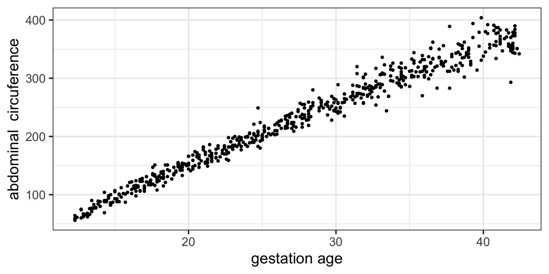
Figure 1: The abdom data.

Fitting Models

library(ggplot2)
library(gamlss.ggplots)
library(gamlss.add)
# Linear
lm1 <- gamlss(y~x, data=abdom, trace=FALSE)
# additive smooth 
am1 <- gamlss(y~pb(x), data=abdom,trace=FALSE)# smooth
# neural network
set.seed(123)
nn1 <- gamlss(y~nn(~x), size=5, data=abdom, trace=FALSE)# neural 
# regression three
rt1 <- gamlss(y~tr(~x),  data=abdom, trace=FALSE)# three
GAIC(lm1, am1, nn1, rt1)

Fitting Models

           df      AIC
am1  6.508274 4948.869
nn1 12.000000 4965.171
lm1  3.000000 5008.453
rt1 14.000000 5305.390

Linear Model

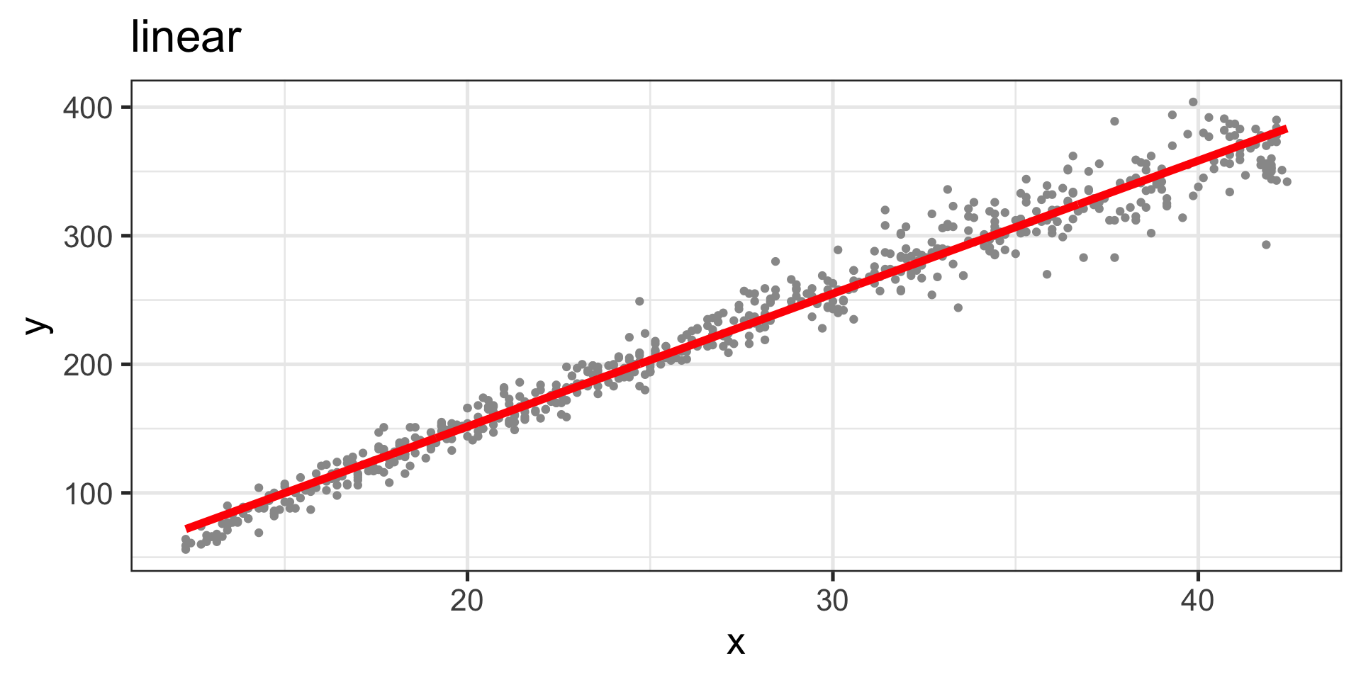
Figure 2: Fitted values, linear curve

Additive Smooth Model

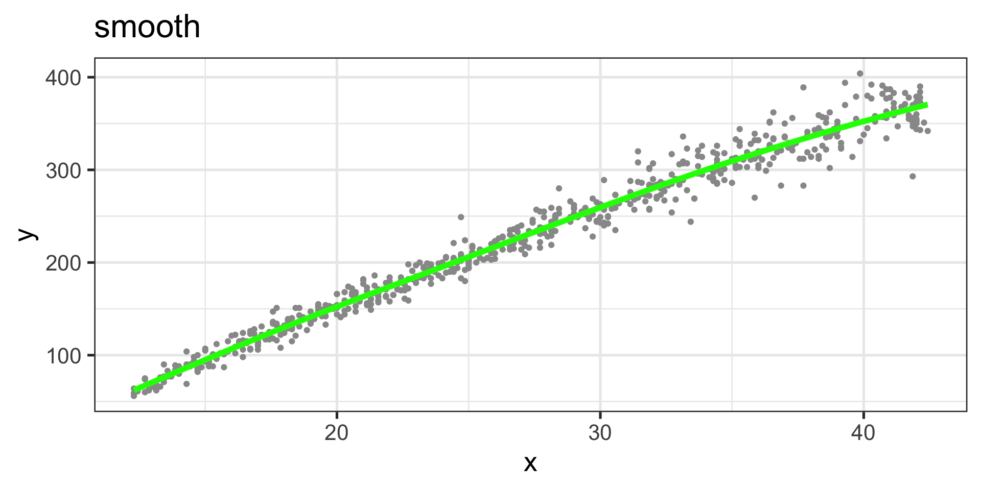
Figure 3: Fitted values, smooth curve

Neural network

Figure 4: Fitted values, neural network curve

Regression Tree

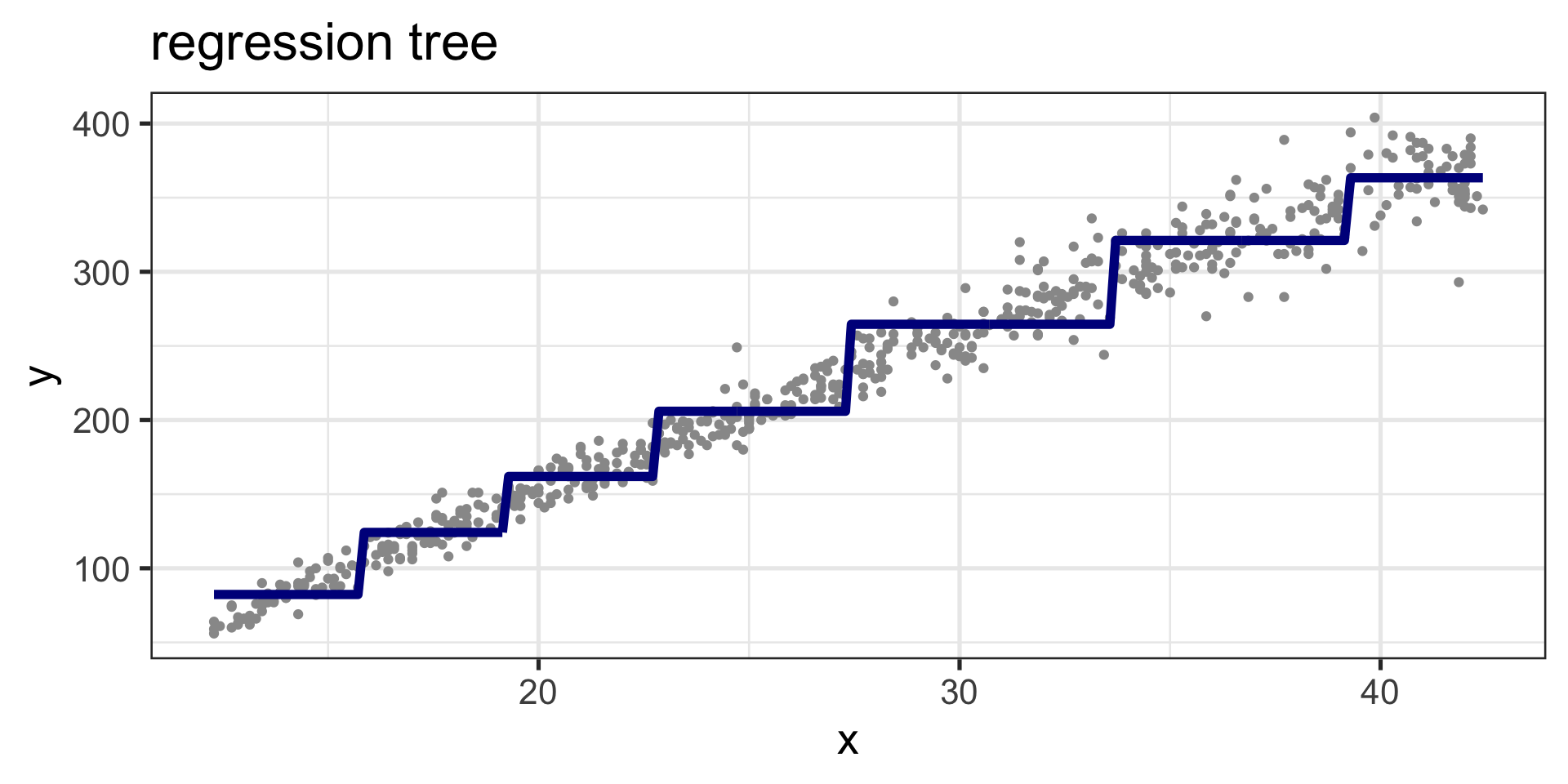
Figure 5: Fitted values, regression tree curve

Diagnostics: QQ plot

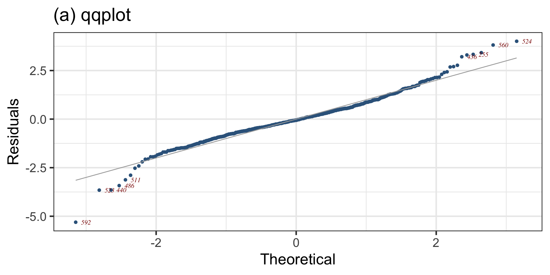
Figure 6: QQ-plot of the fitted am1 model

Diagnostics: Bucket plot

Figure 7: QQ-plot of the fitted am1 model

Refit

am2 <- gamlss(y~pb(x),~pb(x), data=abdom,trace=FALSE)# smooth
 FD <- chooseDist(am2, parallel="snow", ncpus = 10L)

minimum GAIC(k= 2 ) family: ST3 
minimum GAIC(k= 3.84 ) family: LO 
minimum GAIC(k= 6.41 ) family: LO 

am3 <- update(am2, family=LO) 

QQ plot, Logistic

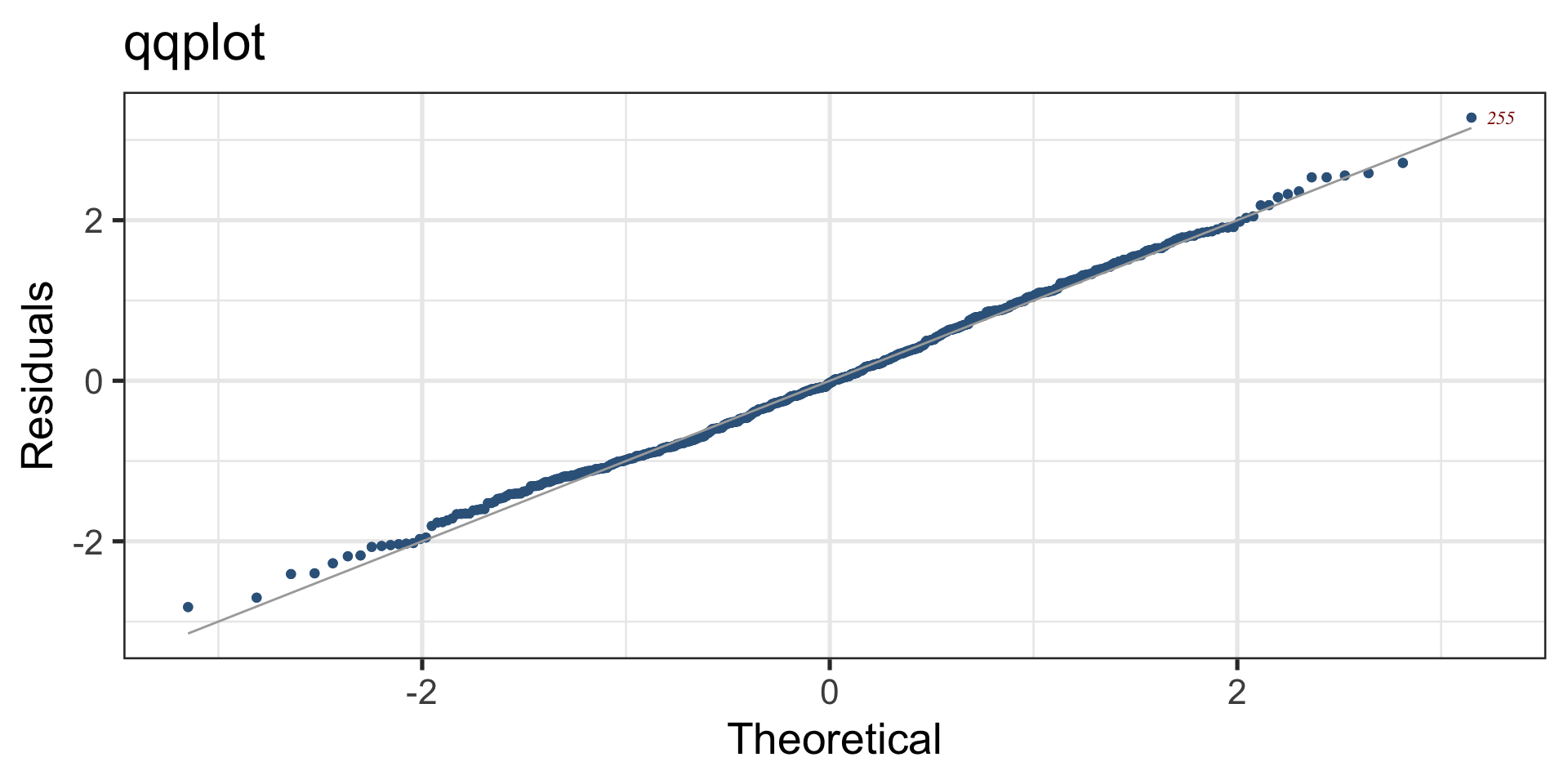
Figure 8: QQ-plot of the fitted am1 model

Bucket plot, Logistic

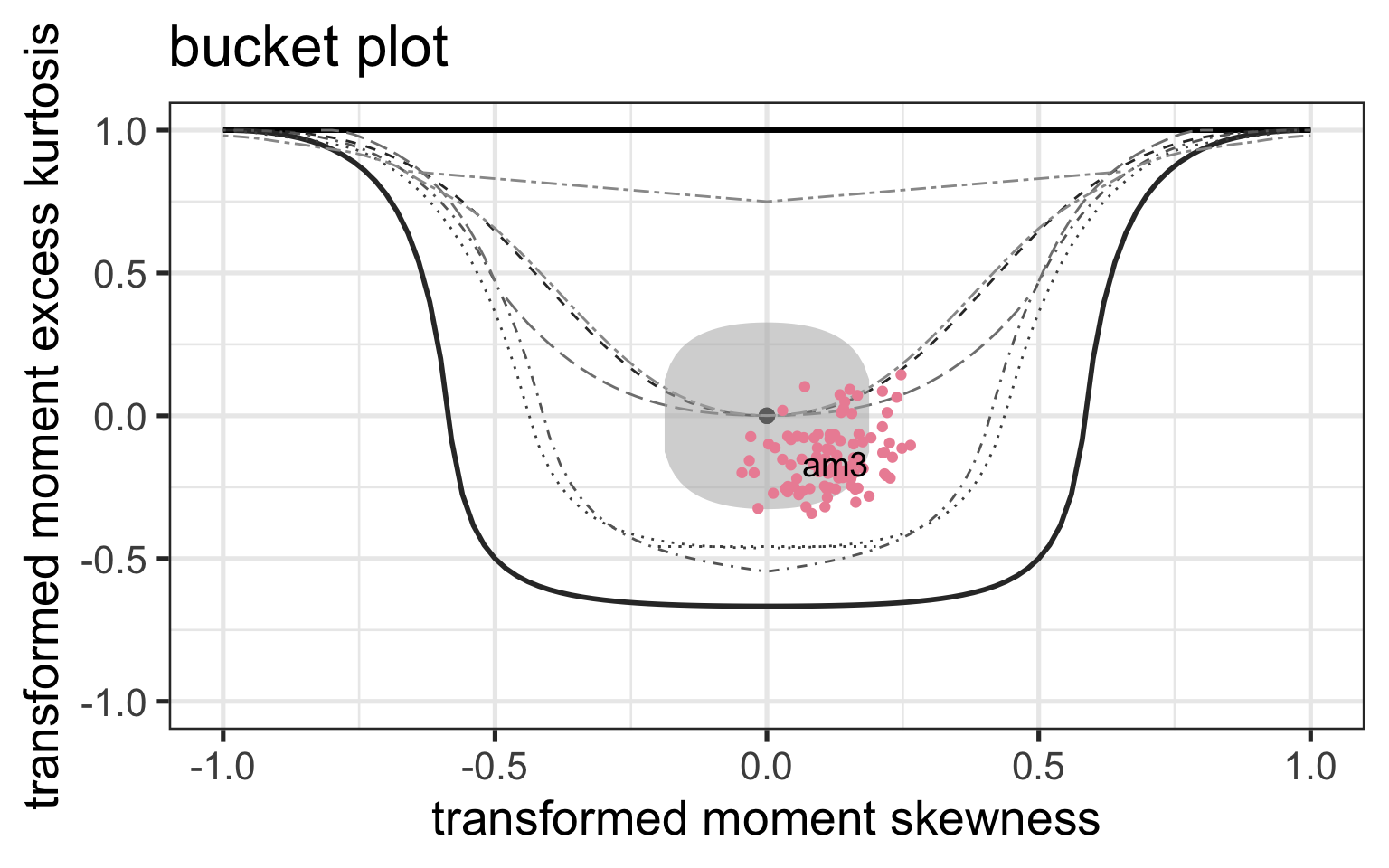
Figure 9: QQ-plot of the fitted am1 model

Fitted Centiles

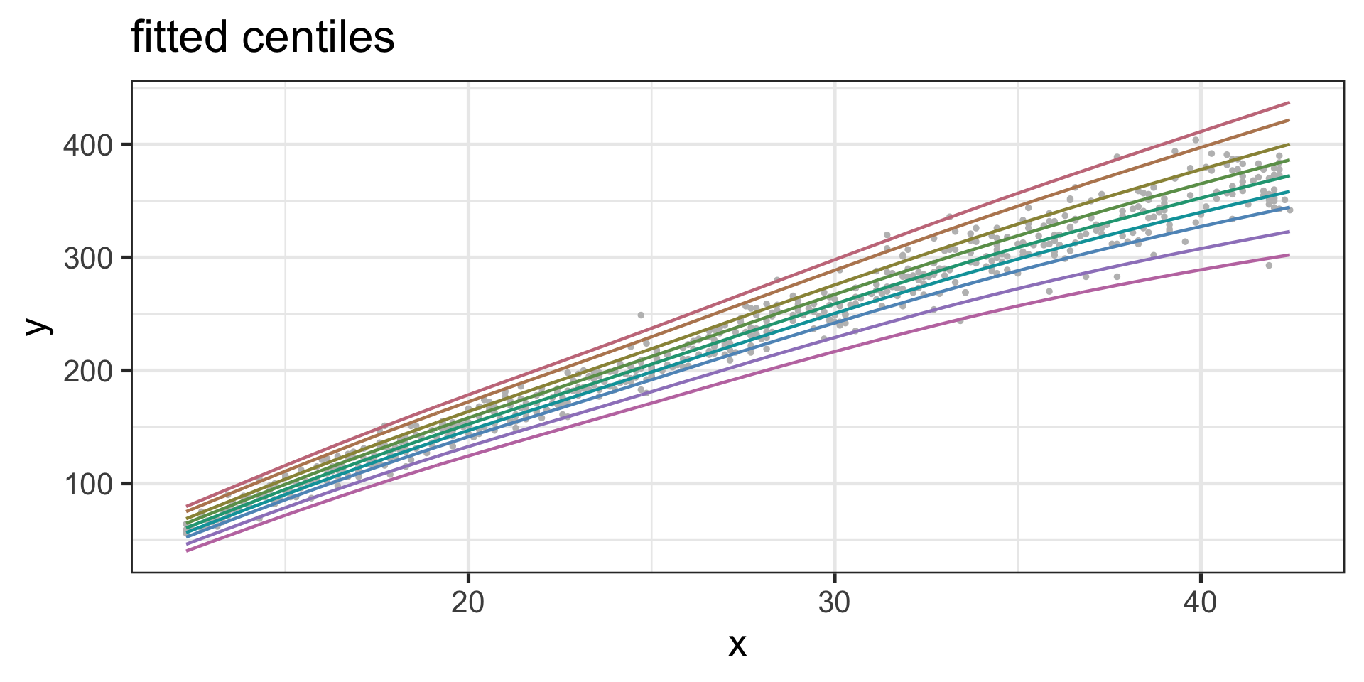
Figure 10: Centile-plot of the fitted am1 model

Fitted Distributions

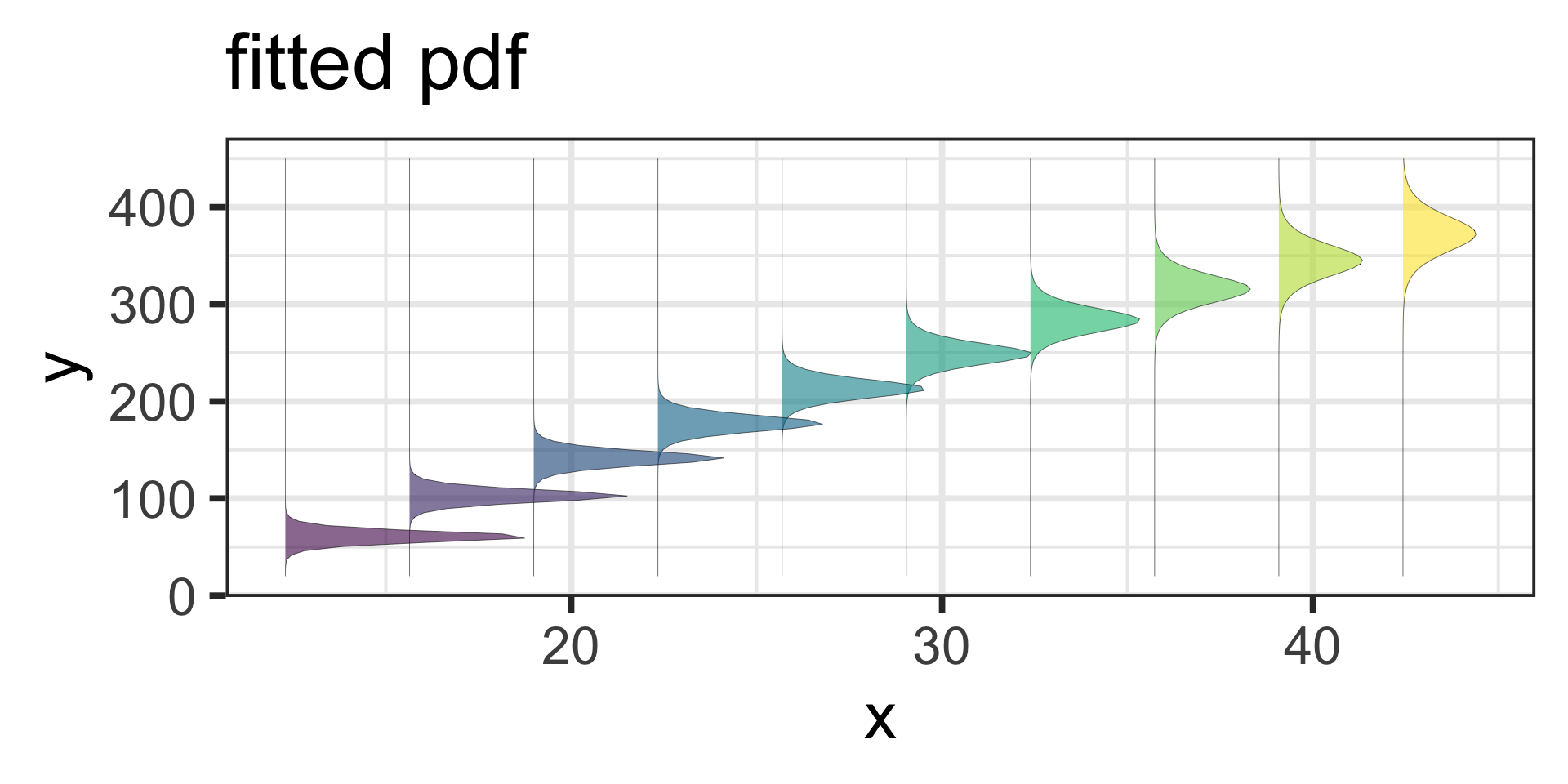
Figure 11: pdf-plot of the fitted am3 model

Summary

• The additive smooth model is the best parsimonious model

• A kurtotic distribution is adequate for the data

• No simple Machine Learning method will do because there is kurtosis and we are interested in centiles

• quantile regression could be used here but in general it is more difficult to check the implicit assumptions made

Tip

Implicit assumptions are more difficult to check

end

back to the index

The Books