Distributions

Mikis Stasinopoulos

Bob Rigby

Fernanda De Bastiani

Introduction

Suitable distribution for the response variable.`

different types of distributions
properies of distributions
a procedure to find a good initial distribution for the response

distributions

Types

continuous
- \((-\infty, \infty)\), real line;
- \((0, \infty)\), positive real line;
- \((0,1)\) from 0 to 1
discrete
- \((0,1,\dots, \infty)\)
- \((0,1,\dots, N)\)
mixed part continuous part discrete
- \([0, \infty)\) zero adjusted
- \([0, 1]\) zero (and 1) inflated

continuous

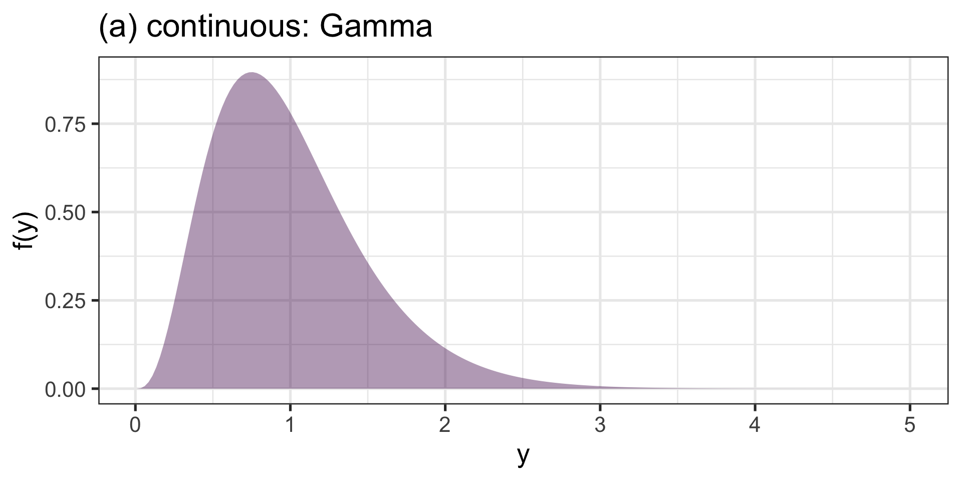
(a) continuous

discrete

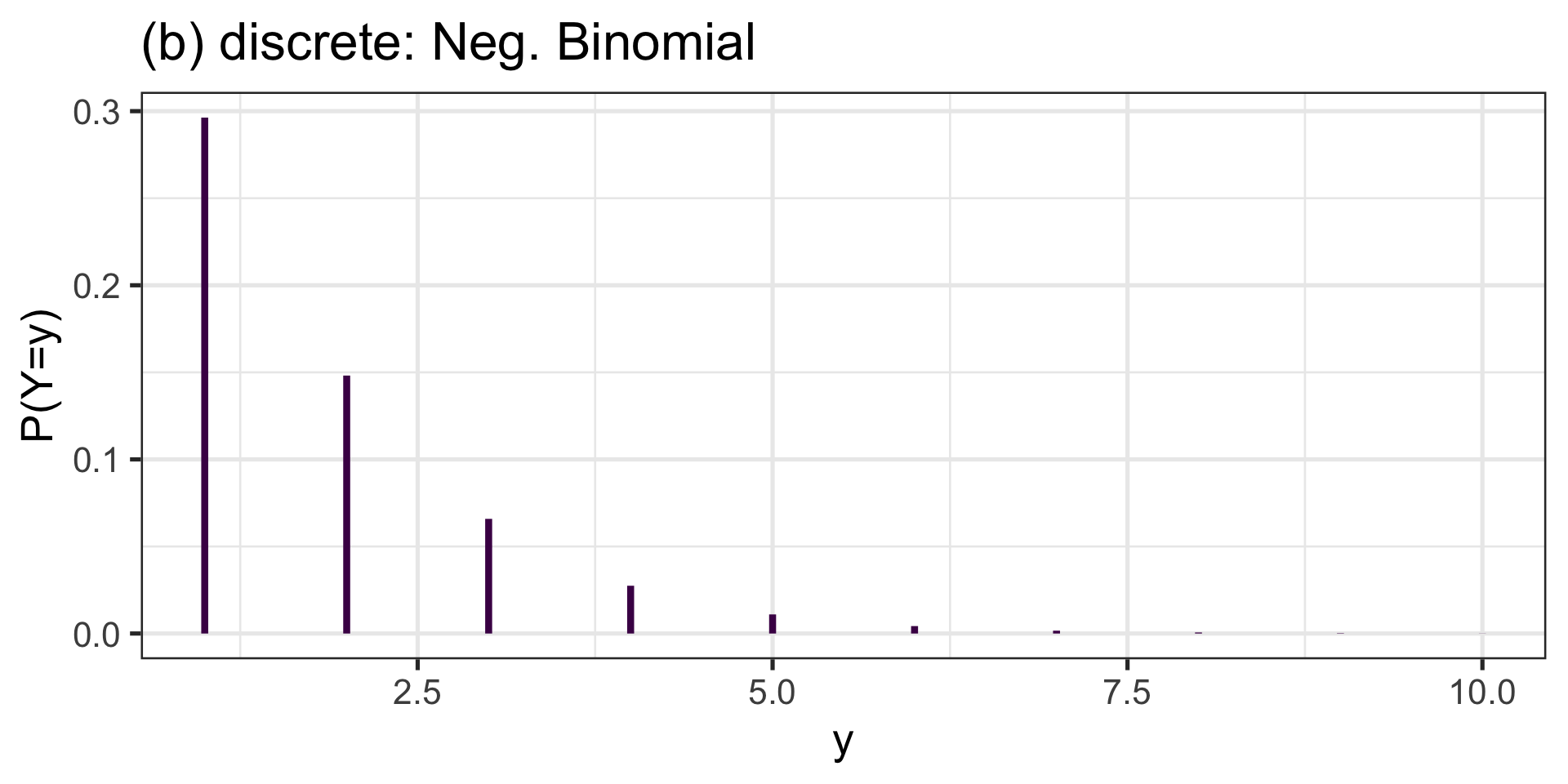
(a) discrete

mixed

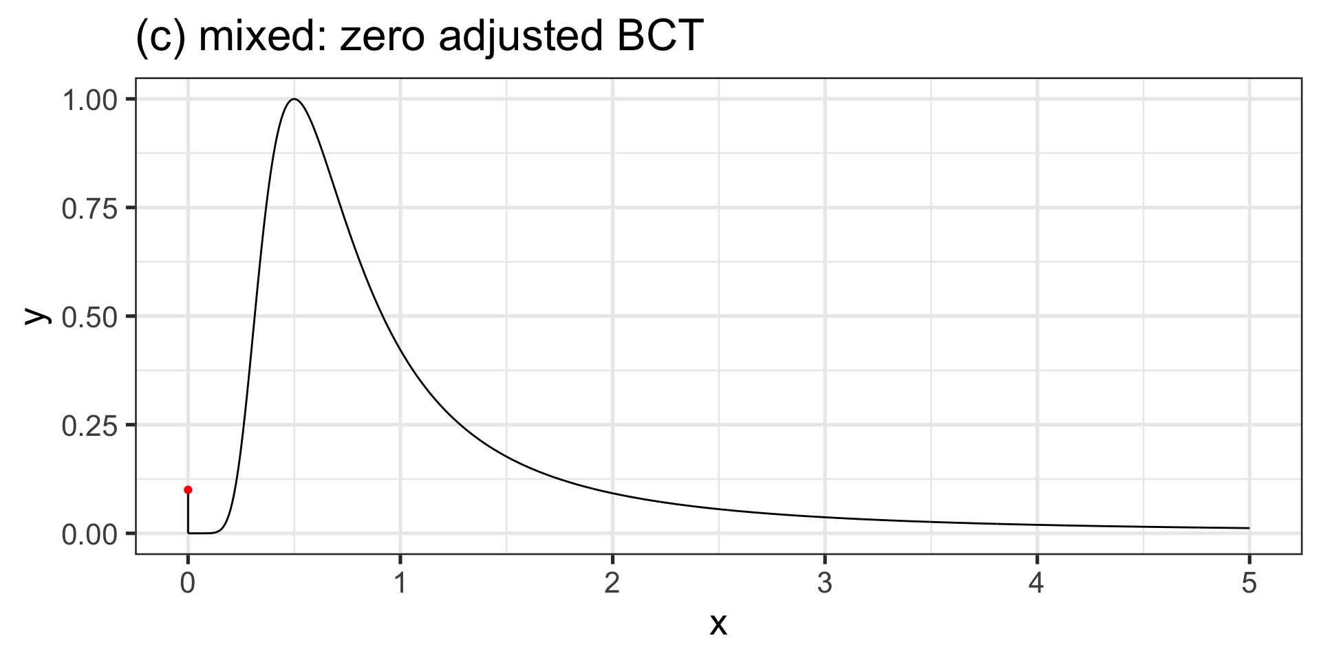
(a) mixed

properties

\(f(y;{\theta})\)

\(\int_{R_Y} f(y) \; dy=1\)
\(\sum_{y\in R_Y} f(y)=\sum_{y \in R_Y} P(Y=y)=1\)
\(\int_{R_{1}} f(y)\, dy + \sum_{y \in R_{2}} f(y) = 1\).

parameters

\(f(y;{\theta})\)
\({\theta}= (\theta_1, \theta_2, \ldots, \theta_k)\).
location
scale
shape
- skewness
- kurtosis

left skew

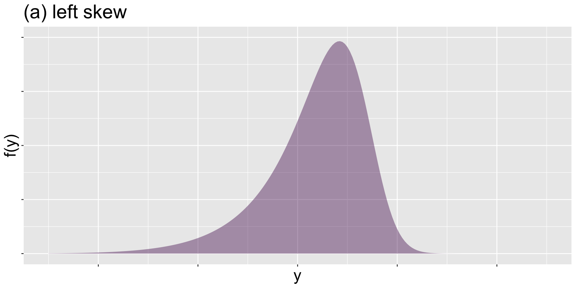
(a) left skew

symmetric

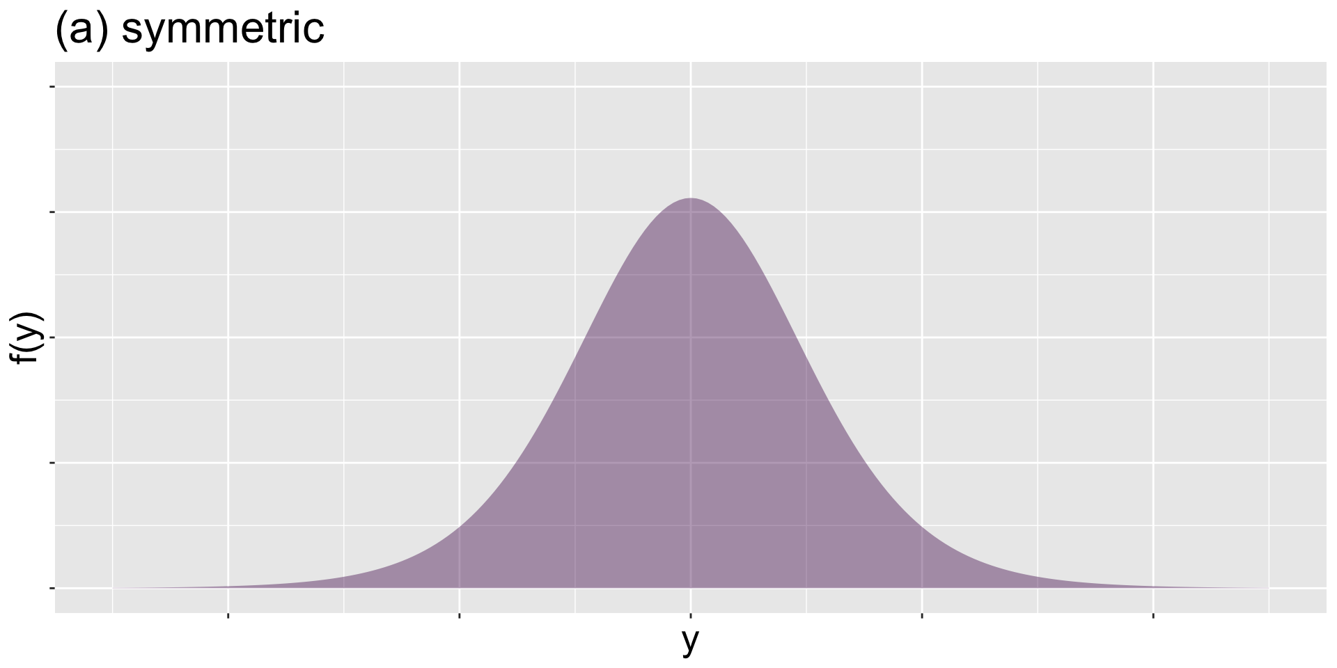
(a) symmetric

right skew

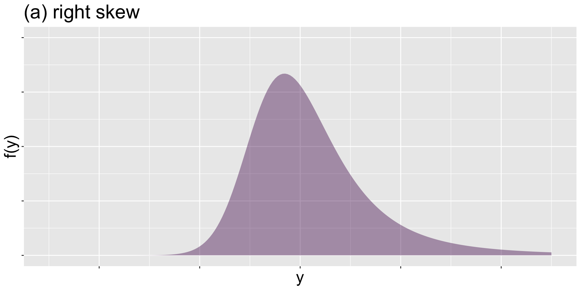
Figure 6: right skew

platy

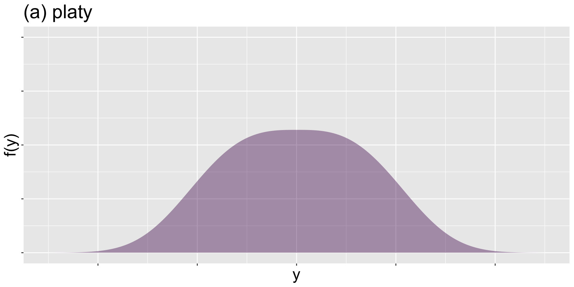
(a) platy

meso

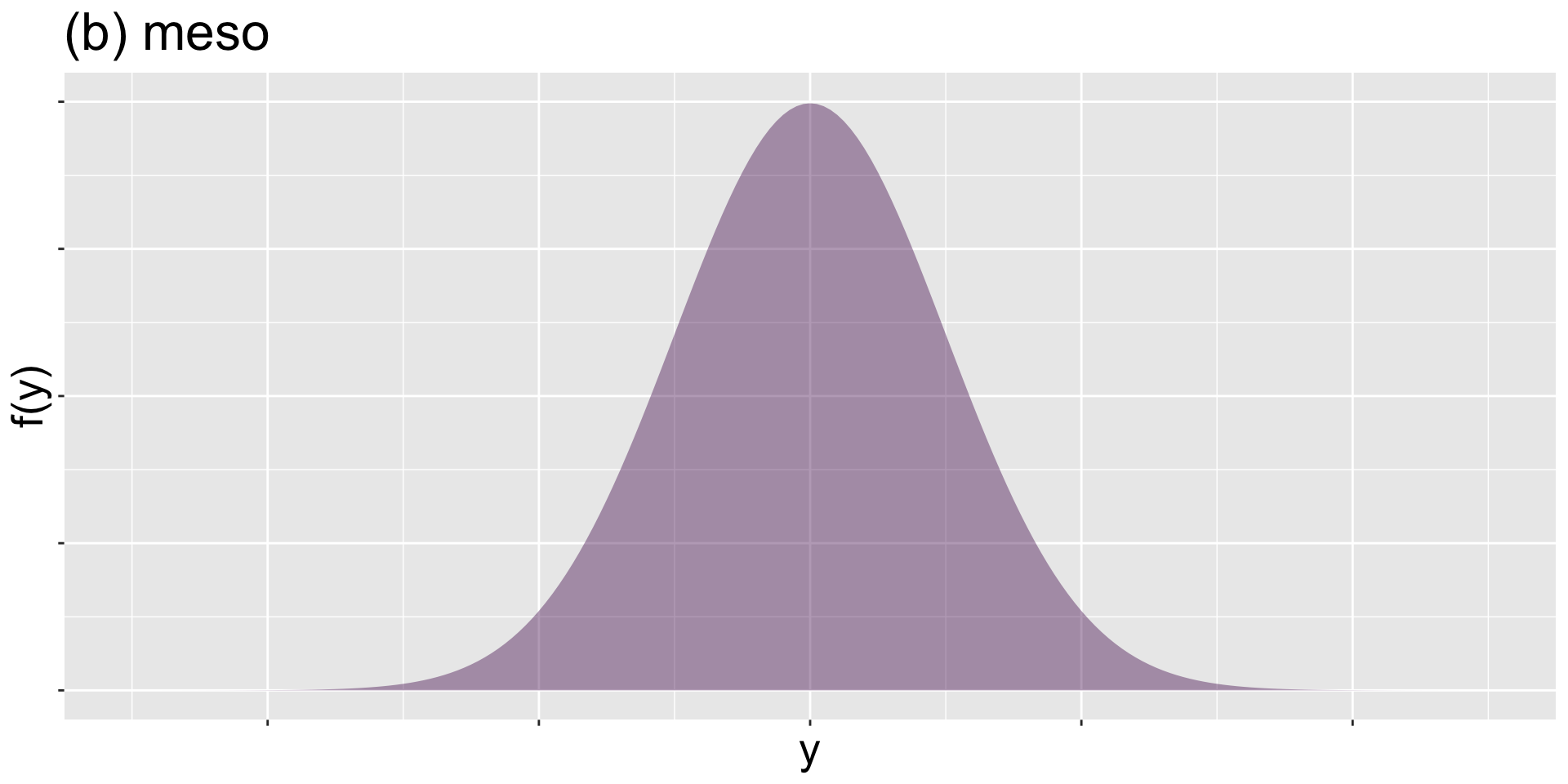
Figure 8: meso

lepto

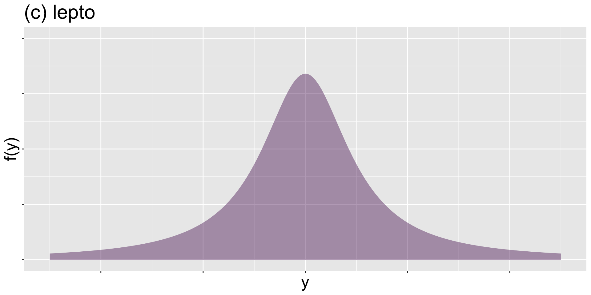
Figure 9: lepto

momments based characteristics

mean \[\begin{align*} E(Y)= \begin{cases} \int_{-\infty}^{\infty} y f(y)\, dy&\text{for continuous}\\ \sum_{y \epsilon R_Y} y\, P(Y=y) &\text{for discrete} \end{cases} \end{align*}\]
variance
coefficient of skewness
(adjusted) coefficient for kurtosis

mean

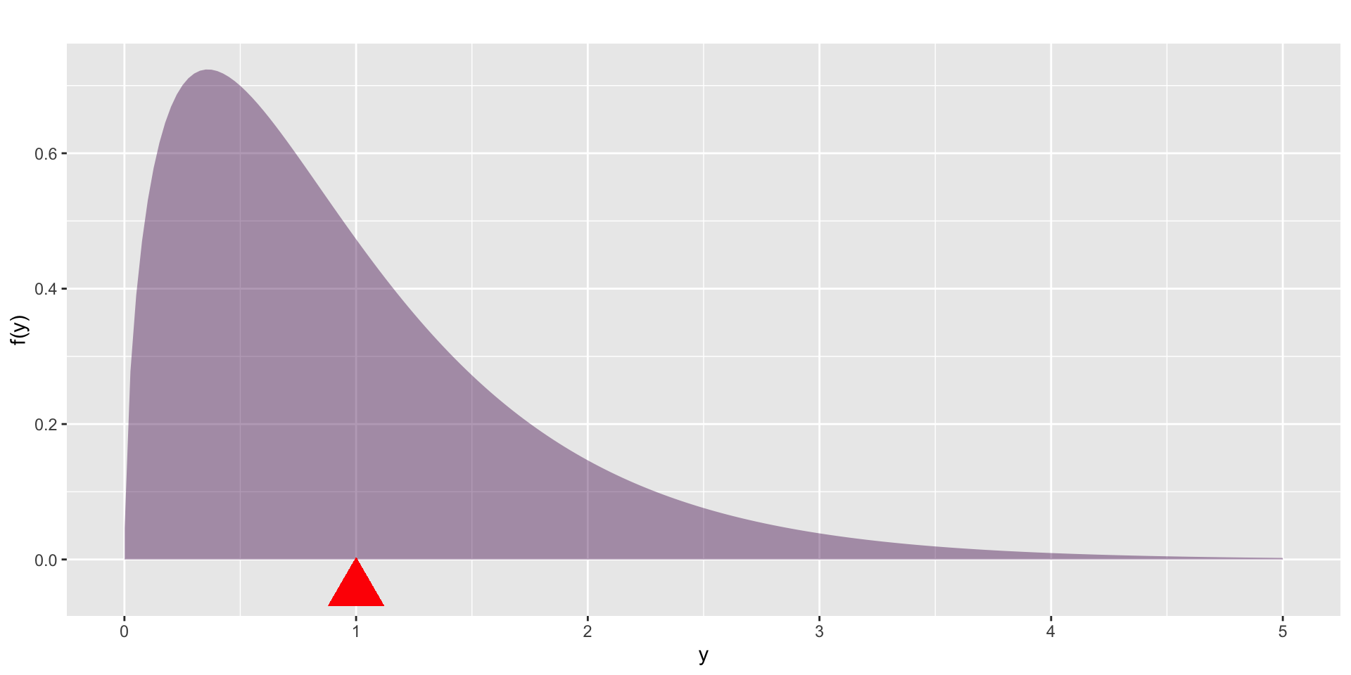
Figure 10: The mean is the point in which the distribution is balance.

centile based characteristics

the median
semi interquartile range
centile skewness
centile kurtosis

quantiles

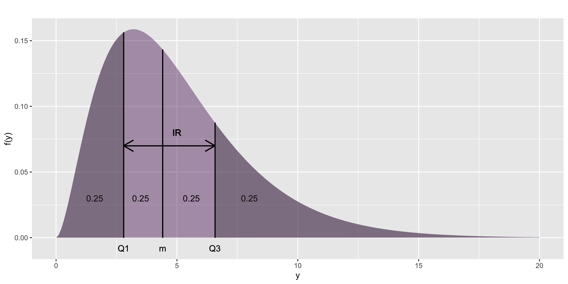
Figure 11: Showing how \(Q1\), \(m\) (median), \(Q3\) and the interquartile range IR of a continuous distribution are derived from \(f(y)\).

The GAMLSS families

over 100 explicit distributions
implicit distributions
- truncation
- log distributions
- logit distribution
- inflated distributions
- zero adjusted
- generalised Tobit

book 2

book2

select distribution

Find a distribution

flowchart TB
  A[responce] --> B(continuous) 
  A --> C[discrete]
  A --> D[factor]
  B --> F[real line]
  B --> G[pos. real line]
  B --> H[0 to 1]
  C --> J[infinite count]
  C --> I[finite count]
  D --> K[unordered]
  D --> L[ordered]
  I --> N[binary]
  K --> N[binary]

Figure 12: Type of distribution for the response.

Summary

Select an appropriate class of distributions following the diagram above.
Use the function chooseDist() to fit a “linear” models for both \(\mu\) and \(\sigma\)
Use GAIC to finds the best fit
Use model diagnostics to ckeck the distribution

`chooseDist()`

da <- rent99[, -c(2,9)]
# fit a linear model with all variables above to both mu and sigma
 m1 <- gamlss(rent~.,~., data=da, family=GA,trace=FALSE)
 M1 <- chooseDist(m1, type="realplus", parallel="snow", ncpus=10)
 getOrder(M1, column=1)

GAIG with k= 2 
    BCTo    BCCGo       BCPEo         GG      GB2     BCCG         
38434.95 38435.45    38436.65  38448.71 38470.43  38474.03

worm plot

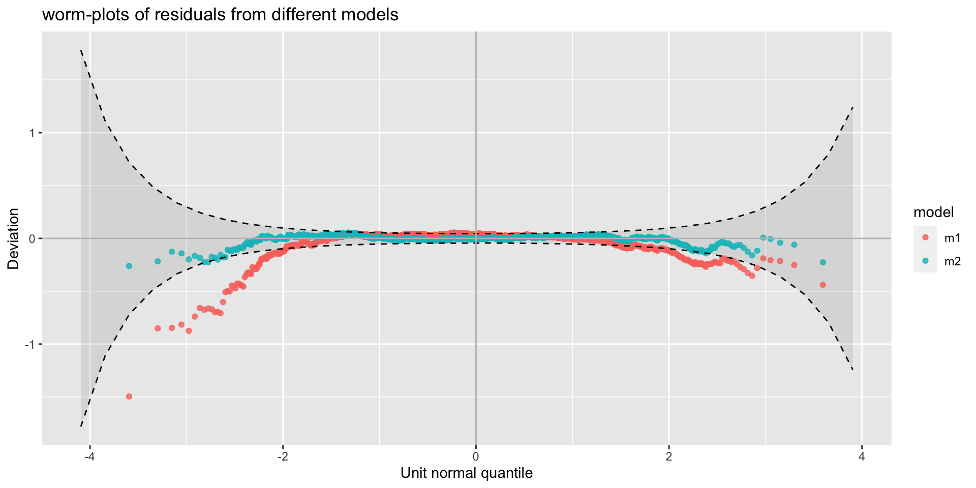
(a) worm plots

bucket plot

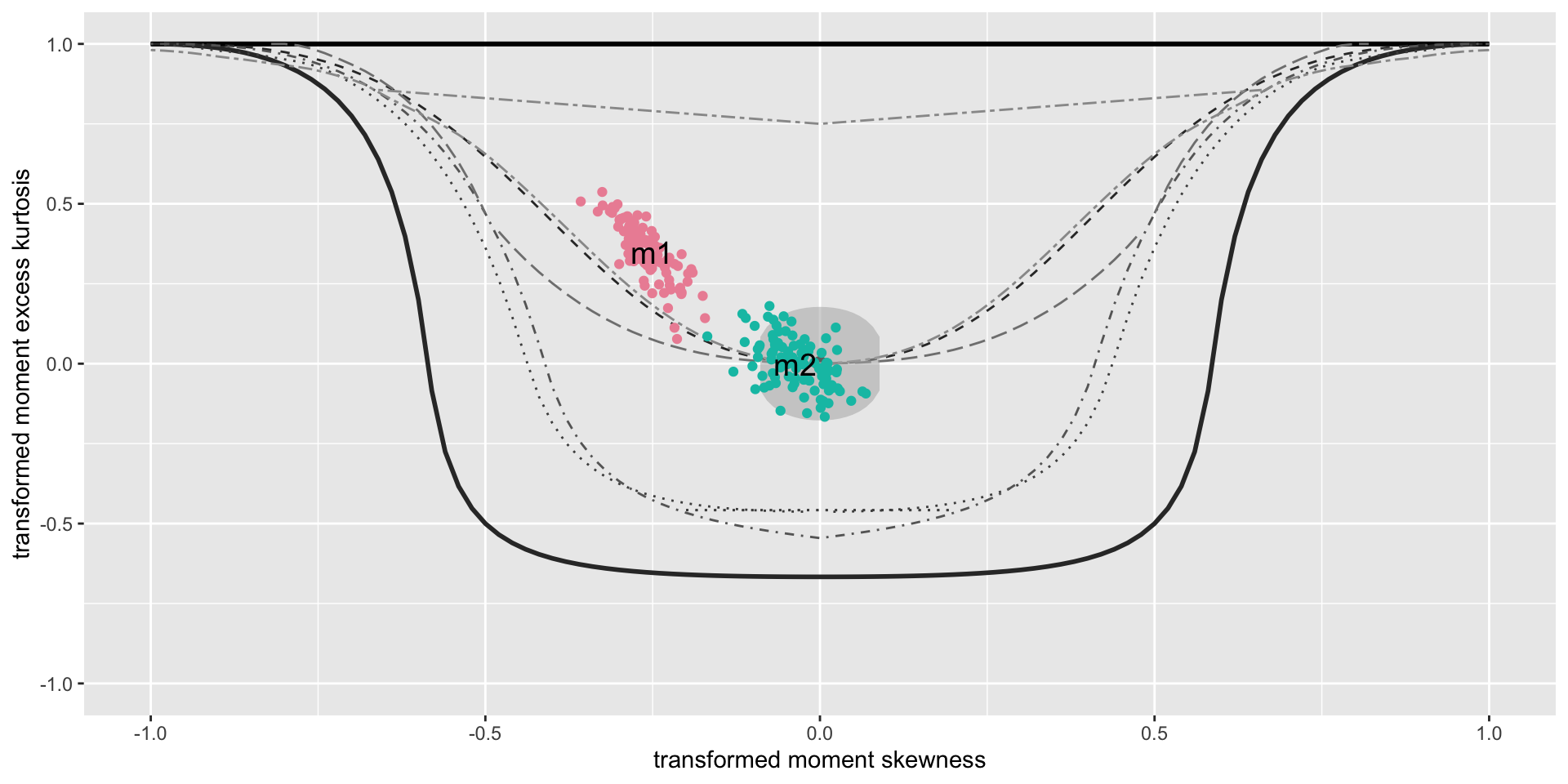
(a) bucket plots

Summary

flowchart TB
  A(responce) --> B[type] 
  B --> C[initial fit]
  C --> D[chooseDist]
  D --> F{check}
  F --> G[residual diagnostics]
  F --> E[overfitting]

Figure 15: Summary for finding an initial distribution.

end

back to the index

The Books