Data

Mikis Stasinopoulos

Bob Rigby

Fernanda De Bastiani

Introduction

• checking the structure of the data

• displaying the data to identify;

  • outliers,
  • possible x-variables transformations,
  • correlation in the feature and
  • possible pair-wise interactions

• partitioning the data

checking the data

Data

Table 1: The Table of Data

obs number	y	x1	x2	x3	…	xr-1	xr
1	y1	x11	x12	x13	…	x1r-1	x1r
2	y2	x21	x22	x23	…	x2r-1	x2r
3	y3	x31	x32	x33	…	x3r-1	x3r
…	…	…	…	…	…	…	…
n-1	yn-1	xn-11	xn-12	xn-12	…	xn-1r-1	xn-1r
n	yn	xn1	xn2	xn3	…	xnr-1	xnr

The rent 1999 Munich data

Table 2: Variables in Munich rent data

rent	area	yearc	location	bath	kitchen	cheating
109.95	26	1918	2	0	0	0
243.28	28	1918	2	0	0	1
261.64	30	1918	1	0	0	1
106.41	30	1918	2	0	0	0
133.38	30	1918	2	0	0	1
339.03	30	1918	2	0	0	1

Important features

• the range of the response variable,

• how explanatory variables should be enter the regression

• the shape of the data

• missing values NA’s

• names of columns

• factors

the range of the response

flowchart TB
  A[responce] --> B(continuous) 
  A --> C[discrete]
  A --> D[factor]
  B --> F[real line]
  B --> G[pos. real line]
  B --> H[0 to 1]
  C --> J[infinite count]
  C --> I[finite count]
  D --> K[unordered]
  D --> L[ordered]
  I --> N[binary]
  K --> N[binary]

Important for determine the distribution

explanatory variables

• continuous
  • linear effect
  • non-linear effect
• factors
  • non ordered
  • ordered
• interactions

data dimension

• data_dim(): information about dimensions

da |> data_dim()

************************************************************** 
************************************************************** 
the dimensions of the data set are: 3082 by 7 
number of observations with missing values; 0 
% data omited; 0 % 
************************************************************** 
************************************************************** 

• data_which_na(): which variables have missing observations

da |> data_which_na()

    rent     area    yearc location     bath  kitchen cheating 
       0        0        0        0        0        0        0 

variable names

• data_names()

da |> data_names()

************************************************************** 
************************************************************** 
the names of variables 
[1] "rent"     "area"     "yearc"    "location" "bath"     "kitchen"  "cheating"
************************************************************** 
************************************************************** 

• `data_sorter_names()’: shortening the names

da |> data_sorter_names( max=10) -> da

************************************************************** 
************************************************************** 
the names of variables 
[1] "rent"     "area"     "yearc"    "location" "bath"     "kitchen"  "cheating"
************************************************************** 
************************************************************** 

missing values

• The gamlss() function can not cope with missing values.

• to deal with NA’s see https://stefvanbuuren.name/fimd/

data shape

(a) \(n<p\) more obstervations than variable (b) \(n>p\) more variables than obsrvations

Factors

• any character vector
• any vector variable with a small range of distinct values,

  (Intercept) x qrt2 qrt3 qrt4
1           1 1    0    0    0
2           1 2    1    0    0
3           1 3    0    1    0
4           1 4    0    0    1
5           1 5    0    0    0
6           1 6    1    0    0
7           1 7    0    1    0
8           1 8    0    0    1

the structure of the data

da |> data_str()

************************************************************** 
************************************************************** 
the structure of the data 
'data.frame':   3082 obs. of  7 variables:
 $ rent    : num  110 243 262 106 133 ...
 $ area    : int  26 28 30 30 30 30 31 31 32 33 ...
 $ yearc   : num  1918 1918 1918 1918 1918 ...
 $ location: Factor w/ 3 levels "1","2","3": 2 2 1 2 2 2 1 1 1 2 ...
 $ bath    : Factor w/ 2 levels "0","1": 1 1 1 1 1 1 1 1 1 1 ...
 $ kitchen : Factor w/ 2 levels "0","1": 1 1 1 1 1 1 1 2 1 1 ...
 $ cheating: Factor w/ 2 levels "0","1": 1 2 2 1 2 2 1 2 1 1 ...
************************************************************** 
************************************************************** 
table of the class of variabes 
class_Vars
 factor integer numeric 
      4       1       2 
************************************************************** 
************************************************************** 
and those integer vectors into mumeric: 
area 
************************************************************** 
************************************************************** 
distinct values in variables 
    rent     area    yearc location     bath  kitchen cheating 
    2723      132       68        3        2        2        2 
************************************************************** 
************************************************************** 

displaying the data

Plotting individual vectors

• data_plot()

Figure 1: Plotting the invidual variables of the data

Plotting individual vectors (1)

• data_bucket()

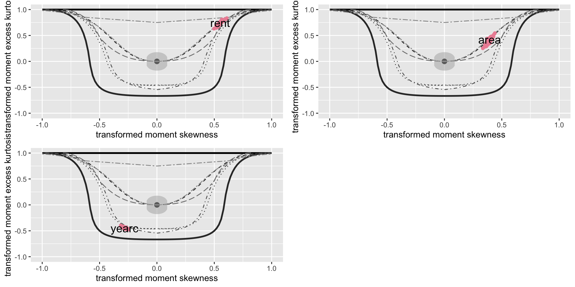
Figure 2: Plotting the bucket plot for the continuous variables in the data

Plotting individual vectors (2)

data_zscores()

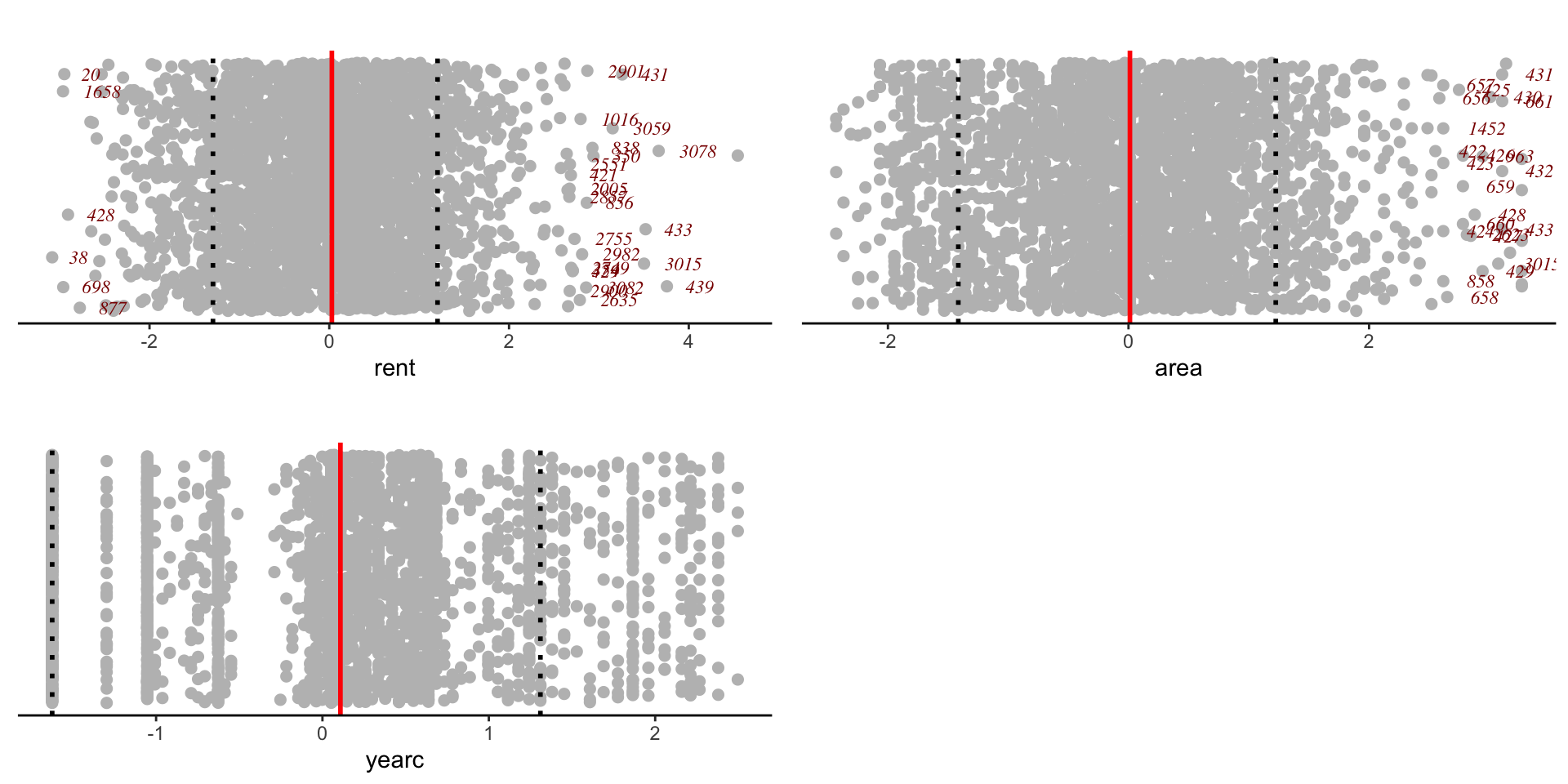
Figure 3: Plotting the histogtams of the continuous variables in the data

z-scores (standardization)

• standardization subtract from the mean and divide by standard deviation (no good for skew and kurtotic data)

• y_zscores(): fits a SHASHo distribution and take the residuals

 z <- y_zscores(da$rent, plot=FALSE) # is equivalent to the steps
m1 <- gamlssML(da$rent, family=SHASHo) # fitting a 4 parameter distribution 
cbind(z,resid(m1))[1:5,]#  and taking the residuals

          z          
1 -2.496097 -2.496097
2 -1.340464 -1.340464
3 -1.182014 -1.182014
4 -2.526326 -2.526326
5 -2.295069 -2.295069

The response variable

the class of the response is numeric is this correct? 
a continuous distribution on (0,inf) could be used 

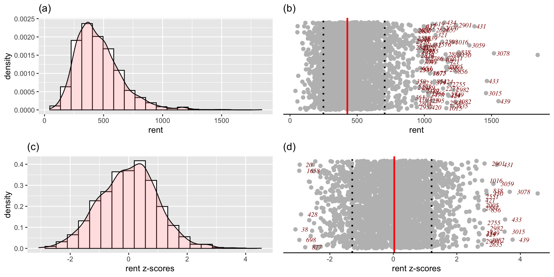
Figure 4: The response variable, (a) histogram of the response variable (b) a dot plot of the response variable (c) histogram of the z-scores of the response variable after standardised using the SHASH distribution (d) a dot plot of the z-scores of response variable.

Pair-wise data plots

Figure 5: The response variable aganst all explanatory variables.

Outliers

• within columns (variables)

• between rows (observations)

Outliers within columns

Algorithm to identify outliers in continuous variables

• Initialize: select all continuous variables \(x_1, x_2,\ldots, x_R\)

• For r in 1 to R

• If \(x_r\) in \(\mathbb{R}^{+}\) find \(p\) to transform \(x_r\) using the power transformormation, \(y_r = x_r^p\) for \((0 \le p < 1.5)\) else set \(y_r=x_r\). EndIf

• standardised \(y_r\) to \(z_r\) using a sinh-archsinh transformation and get the z-scores

• identify z-scores with absolute value greater that a predetermine value \(|z_r| > \text{val}\) i.e. 4

• EndFor

• print the identified observations

Outliers within columns (2)

• data_outliers()

 gamlss.ggplots:::data_outliers(da)

$rent
named numeric(0)

$area
named integer(0)

$yearc
named numeric(0)

Outliers between rows

• data_leverage()

gamlss.ggplots:::data_leverage(da, response=rent)

Figure 6: The observations against the linear leverage.

Transformation of variables

• transformation for skew x-variables to be transformed into a more evenly spaced. A power transformation of the type \(x^p\) for \(0<p<1\), where p=0 usualy is defines as \(\log(x)\).

• standardisation is needed to make sure that at least all continuous explanatory variables would be in a similar scale

  • z-scores
  • 0 to 1

Transformation

• data_trans()

Figure 7: The response against linear the continuous variables: on the left have no transformation, in the middle the square root ; on the right log

standardisation

• data_stad()

      rent       area yearc location bath kitchen cheating
1 109.9487 0.04285714     0        2    0       0        0
2 243.2820 0.05714286     0        2    0       0        1
3 261.6410 0.07142857     0        1    0       0        1
4 106.4103 0.07142857     0        2    0       0        0
5 133.3846 0.07142857     0        2    0       0        1
6 339.0256 0.07142857     0        2    0       0        1

pair-wise linear correlations

gamlss.ggplots:::data_cor(da, method="square")

4 factors have been omited from the data 

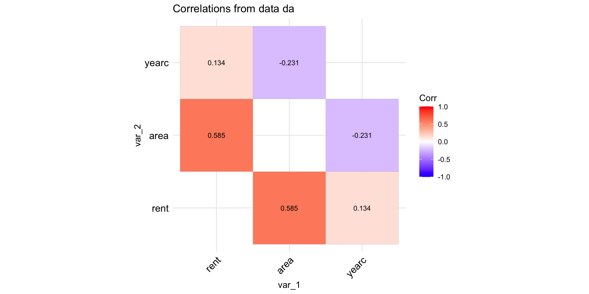
Figure 8: The linear correlation coefficients of the continuous variables in the data

pair-wise interactions

da |> gamlss.ggplots:::data_inter(response= rent)

Figure 9: The pair wise interaction plots.

partitioning the data

partitioning tha data

• 2-sections: training and test;

• 3-sections: training, validation and test ;

• K-sections: for K-fold cross validation;

• bootstrapping.

• why: to get extra information by reusing or splitting the data.

partitioning tha data (con.)

flowchart TB
  A[Data] --> B{Reuse} 
  A --> C{Split}
  C --> D[Training]
  D --> E[Validate]
  E --> O[Test]
  B --> F(Rearranged)
  B --> G(Reweighed)
  G--> H(Bayesian \n Bootstrap)
  G--> J(Boosting)
  F --> K(Non-param. \n Bootstrap)
  F --> L(Cross \n Validation)
  L --> M(k-Fold) 
  L --> N(LOO) 

Figure 10: Different ways of splitting data to get more information”

partitioning tha data (con.)

• the function data_part()

dap <- gamlss.ggplots:::data_part(da)

data partition into two sets 

head(dap)

      rent area yearc location bath kitchen cheating partition
1 109.9487   26  1918        2    0       0        0     train
2 243.2820   28  1918        2    0       0        1      test
3 261.6410   30  1918        1    0       0        1     train
4 106.4103   30  1918        2    0       0        0      test
5 133.3846   30  1918        2    0       0        1      test
6 339.0256   30  1918        2    0       0        1     train

daTrain <- subset(dap, partition=="train")
daTest <- subset(dap, partition=="test")
dim(daTrain)

[1] 1846    8

dim(daTest)

[1] 1236    8

Summary

flowchart LR
  A[data] --> B(size, names, missing) 
  B --> C[factors]
  C --> D{display}
  D --> E[variable plots]
  D --> F[response]
  D --> G[xy-plots]
  F --> J{outliers}
  E --> J
  G --> J
  J <--> K[transformation of x]
  J <--> L[standardization of x]
  K --> M[correlation]
  L --> M  
  M <--> N[interactions]
  N x--x O[partition] 

end

back to the index

The Books

[back](data.qmd)