flowchart LR A[GAMLSS] --> L[Parametric] A --> N[Smooth] L --> B(Likelihood) L --> D(Bayesian) L --> E(Boosting) N --> C(Penalised Likelihood) N --> D(Bayesian) N --> E(Boosting) B --> G[beta's] C --> F[beta's, gamma's, & lambda's] E --> F D --> F D --> G E --> G
Fitting models
Mikis Stasinopoulos
Bob Rigby
Fernanda De Bastiani
Gillian Heller
Niki Umlauf
Introduction
questions
do my data support a GAMLSS model?
do I need GAMLSS to answer my questions?
size of the data
questions of interest
this talk
the basic GAMLSS algorithmdifferent statistical approaches for fitting a GAMLSS modeldifferent machine learning techniques for fitting a GAMLSS model.
Algorithms
GAMLSS
\[\begin{split} y_i & \stackrel{\small{ind}}{\sim }& {D}( \theta_{1i}, \ldots, \theta_{ki}) \nonumber \\ g(\theta_{1i}) &=& b_{10} + s_1({x}_{1i}) + \ldots, s_p({x}_{pi}) \nonumber\\ \ldots &=& \ldots \nonumber\\ g({\theta}_{ki}) &=& b_0 + s_1({x}_{1i}) + \ldots, s_p({x}_{pi}) \end{split} \qquad(1)\]
GAMLSS + ML
\[\begin{split} y_i & \stackrel{\small{ind}}{\sim }& {D}( \theta_{1i}, \ldots, \theta_{ki}) \nonumber \\ g({\theta}_{1i}) &=& {ML}_1({x}_{1i},{x}_{2i}, \ldots, {x}_{pi}) \nonumber \\ \ldots &=& \ldots \nonumber\\ g({\theta}_{ki}) &=& {ML}_1({x}_{1i},{x}_{2i}, \ldots, {x}_{pi}) \end{split} \qquad(2)\]
Parameters for Estimation
distribution parameters
coefficient parameters
  - **coefficients**

  - **random effects**
hyper-parameters
flowchart
The Basic Algorithm for GAMLSS
- For specified distribution family, data and machine learning (ML) model.
Initialize: set starting values for all distribution parameters \((\hat{\boldsymbol{\mu}}^{(0)}, \hat{\boldsymbol{\sigma}}^{(0)}, \hat{\boldsymbol{\nu}}^{(0)}, \hat{\boldsymbol{\tau}}^{(0)} )\).
For i in \(1,2,\ldots\)
fix \(\hat{\boldsymbol{\sigma}}^{(i-1)}\),\(\hat{\boldsymbol{\nu}}^{(i-1)}\), and \(\hat{\boldsymbol{\tau}}^{(i-1)}\) and fit a ML model to iterative response \(\textbf{y}_{\mu}\) using iterative weights \(\textbf{w}_{\mu}\) to obtain the new \(\hat{\boldsymbol{\mu}}^{(i)}\)
fix \(\hat{\boldsymbol{\mu}}^{(i)}\),\(\hat{\boldsymbol{\nu}}^{(i-1)}\), and \(\hat{\boldsymbol{\tau}}^{(i-1)}\) and fit a ML model to iterative response \(\textbf{y}_{\sigma}\) using iterative weights \(\textbf{w}_{\sigma}\) to obtain the new \(\hat{\boldsymbol{\sigma}}^{(i)}\)
fix \(\hat{\boldsymbol{\mu}}^{(i)}\),\(\hat{\boldsymbol{\sigma}}^{(i)}\), and \(\hat{\boldsymbol{\tau}}^{(i-1)}\) and fit a ML model to iterative response \(\textbf{y}_{\nu}\) using iterative weights \(\textbf{w}_{\nu}\) to obtain the new \(\hat{\boldsymbol{\nu}}^{(i)}\)
fix \(\hat{\boldsymbol{\mu}}^{(i)}\),\(\hat{\boldsymbol{\sigma}}^{(i)}\), and \(\hat{\boldsymbol{\nu}}^{(i)}\) and fit a ML model to iterative response \(\textbf{y}_{\tau}\) using iterative weights \(\textbf{w}_{\tau}\) to obtain the new \(\hat{\boldsymbol{\nu}}^{(i)}\)
check if the global deviance, \(-2(\textit{log-likelihood})\) does not change repeat otherwise exit
Important
assumed distribution (the log-likelihood is needed and the first and second derivatives)
hierarchy of the paramerers (i.e. a good location model is required before model the scale)
orthogonality of the parameters (leads to better convergence)
Checking orthogonality
Specify a distribution family, and select values for all the parameters.
generate a sample of of N observations (default \(N=10000\))
fit the distribution to the generated sample.
display the correlation coefficients of the estimated predictors, \(\eta_{\theta}\).
Checking orthogonality (con.)
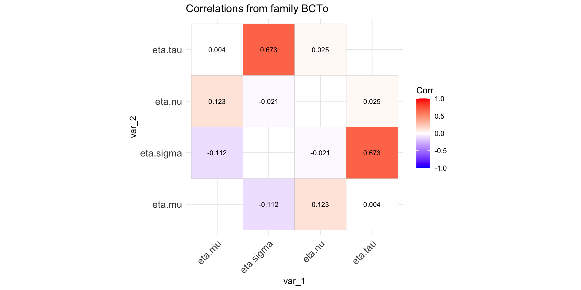
Figure 2: Paramater orthogonality for BCTo distribution
Machine Learning Models
properties
are the standard errors available?
do the x’s need standardization.
about the algorithm
 - stability
 - speed
 - convergence
nonlinear terms
interactions
dataset type
is the selection of x’s automatic?
interpretation
Linear Models
Linear Models
Call:
gamlss2(formula = rent ~ area + poly(yearc, 2) + location + bath +
    kitchen + cheating | area + yearc + location + bath + kitchen +
    cheating, data = da, family = BCTo, ... = pairlist(trace = FALSE))
---
Family: BCTo
Link function: mu = log, sigma = log, nu = identity, tau = log
*--------
Parameter: mu
---
Coefficients:
                 Estimate Std. Error t value Pr(>|t|)
(Intercept)     5.0132864  0.0275445 182.007  < 2e-16 ***
area            0.0106293  0.0002329  45.640  < 2e-16 ***
location2       0.0878750  0.0104118   8.440  < 2e-16 ***
location3       0.1983303  0.0383017   5.178 2.39e-07 ***
bath1           0.0415152  0.0206509   2.010   0.0445 *
kitchen1        0.1129557  0.0236130   4.784 1.80e-06 ***
cheating1       0.3304758  0.0240475  13.743  < 2e-16 ***
poly(yearc, 2)1 5.0471663  0.3301520  15.287  < 2e-16 ***
poly(yearc, 2)2 3.3575299  0.2751069  12.204  < 2e-16 ***
*--------
Parameter: sigma
---
Coefficients:
              Estimate Std. Error   t value Pr(>|t|)
(Intercept)  1.047e+01  6.245e-02   167.650  < 2e-16 ***
area         1.218e-03  6.099e-04     1.996   0.0460 *
yearc       -5.972e-03  8.078e-07 -7392.764  < 2e-16 ***
location2    5.971e-02  2.911e-02     2.051   0.0403 *
location3    2.176e-01  9.224e-02     2.359   0.0184 *
bath1        5.069e-03  5.966e-02     0.085   0.9323
kitchen1     3.750e-02  7.106e-02     0.528   0.5977
cheating1   -2.431e-01  4.766e-02    -5.100  3.6e-07 ***
*--------
Parameter: nu
---
Coefficients:
            Estimate Std. Error t value Pr(>|t|)
(Intercept)  0.65342    0.05454   11.98   <2e-16 ***
*--------
Parameter: tau
---
Coefficients:
            Estimate Std. Error t value Pr(>|t|)
(Intercept)  3.18974    0.01758   181.4   <2e-16 ***
---
Signif. codes:  0 '***' 0.001 '**' 0.01 '*' 0.05 '.' 0.1 ' ' 1
*--------
n = 3082 df =  19 res.df =  3063
Deviance = 38254.617 Null Dev. Red. = 5.95%
AIC = 38292.617 elapsed =  0.32sec
Additive Models
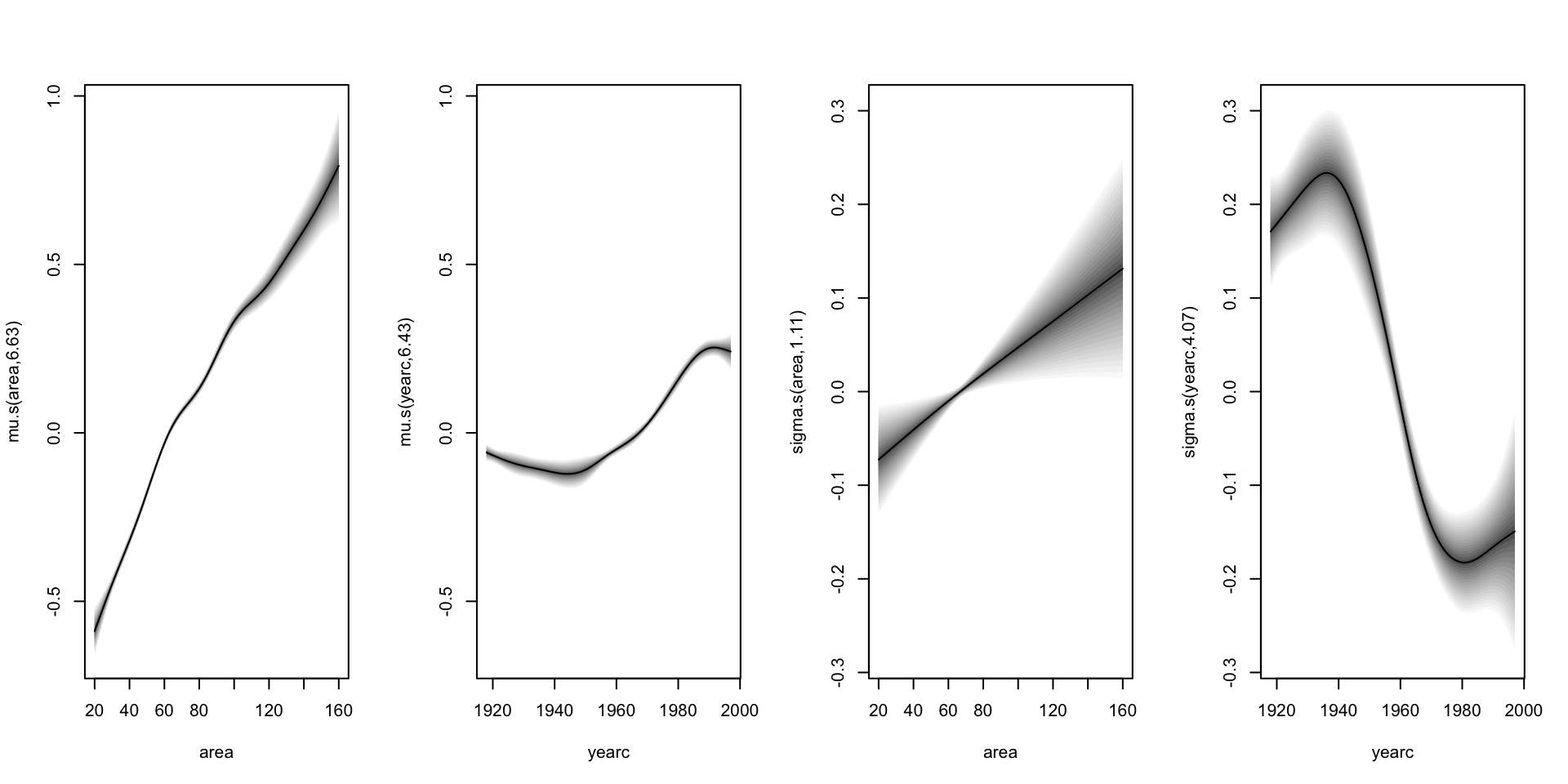
Additive Models (con.)
Call:
gamlss2(formula = rent ~ s(area) + s(yearc) + location + bath +
    kitchen + cheating | s(area) + s(yearc) + location + bath +
    kitchen + cheating, data = da, family = BCTo, ... = pairlist(trace = F))
---
Family: BCTo
Link function: mu = log, sigma = log, nu = identity, tau = log
*--------
Parameter: mu
---
Coefficients:
            Estimate Std. Error t value Pr(>|t|)
(Intercept)  5.71524    0.02082 274.541  < 2e-16 ***
location2    0.08808    0.01102   7.994 1.83e-15 ***
location3    0.20998    0.04965   4.229 2.41e-05 ***
bath1        0.05792    0.04280   1.353  0.17605
kitchen1     0.10859    0.03642   2.982  0.00289 **
cheating1    0.34594    0.02021  17.114  < 2e-16 ***
---
Smooth terms:
    s(area) s(yearc)
edf  6.6271   6.4275
*--------
Parameter: sigma
---
Coefficients:
            Estimate Std. Error t value Pr(>|t|)
(Intercept) -1.15569    0.03695 -31.277  < 2e-16 ***
location2    0.05293    0.02264   2.338   0.0195 *
location3    0.21218    0.08616   2.463   0.0138 *
bath1        0.03440    0.08318   0.414   0.6792
kitchen1     0.01861    0.07591   0.245   0.8063
cheating1   -0.23431    0.03754  -6.242 4.91e-10 ***
---
Smooth terms:
    s(area) s(yearc)
edf  1.1077   4.0742
*--------
Parameter: nu
---
Coefficients:
            Estimate Std. Error t value Pr(>|t|)
(Intercept)  0.69275    0.04548   15.23   <2e-16 ***
*--------
Parameter: tau
---
Coefficients:
            Estimate Std. Error t value Pr(>|t|)
(Intercept)  3.26960    0.07549   43.31   <2e-16 ***
---
Signif. codes:  0 '***' 0.001 '**' 0.01 '*' 0.05 '.' 0.1 ' ' 1
*--------
n = 3082 df =  32.24 res.df =  3049.76
Deviance = 38132.48 Null Dev. Red. = 6.25%
AIC = 38196.9528 elapsed =  0.47sec
Additive Models (con.)
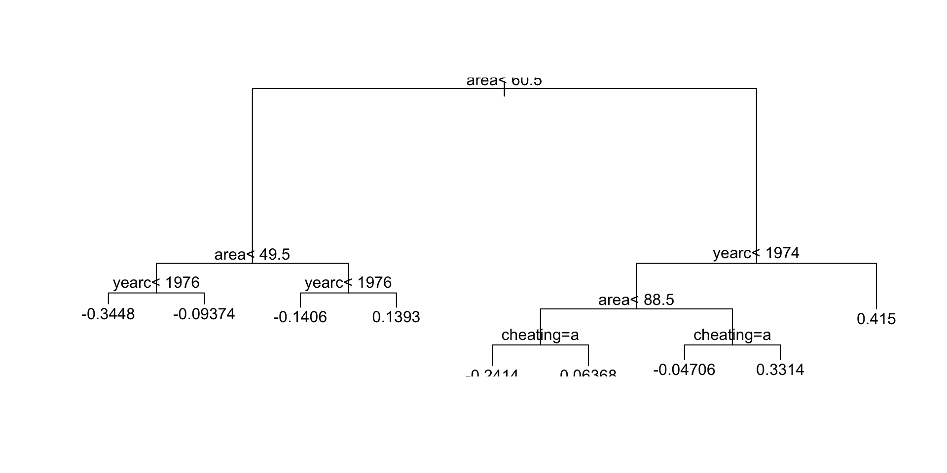
Regression Trees
source("~/Dropbox/GAMLSS-development/nnet/reg.tree.R")
mregtree <- gamlss2(rent~tree(~area+yearc+location+bath+kitchen+cheating)|
                       tree(~area+yearc+location+bath+kitchen+cheating),
                  family=BCTo, data=da, trace=FALSE)

GAIC(mlinear, madditive, mregtree)
AIC df
madditive 38196.95 32.2364
mlinear 38292.62 19.0000
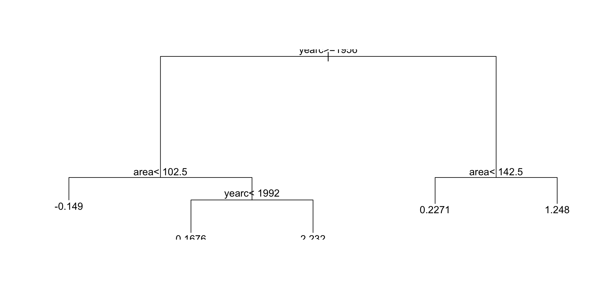
mregtree 38754.64 30.0000Regression Trees (con.)
Regression Trees (continue)
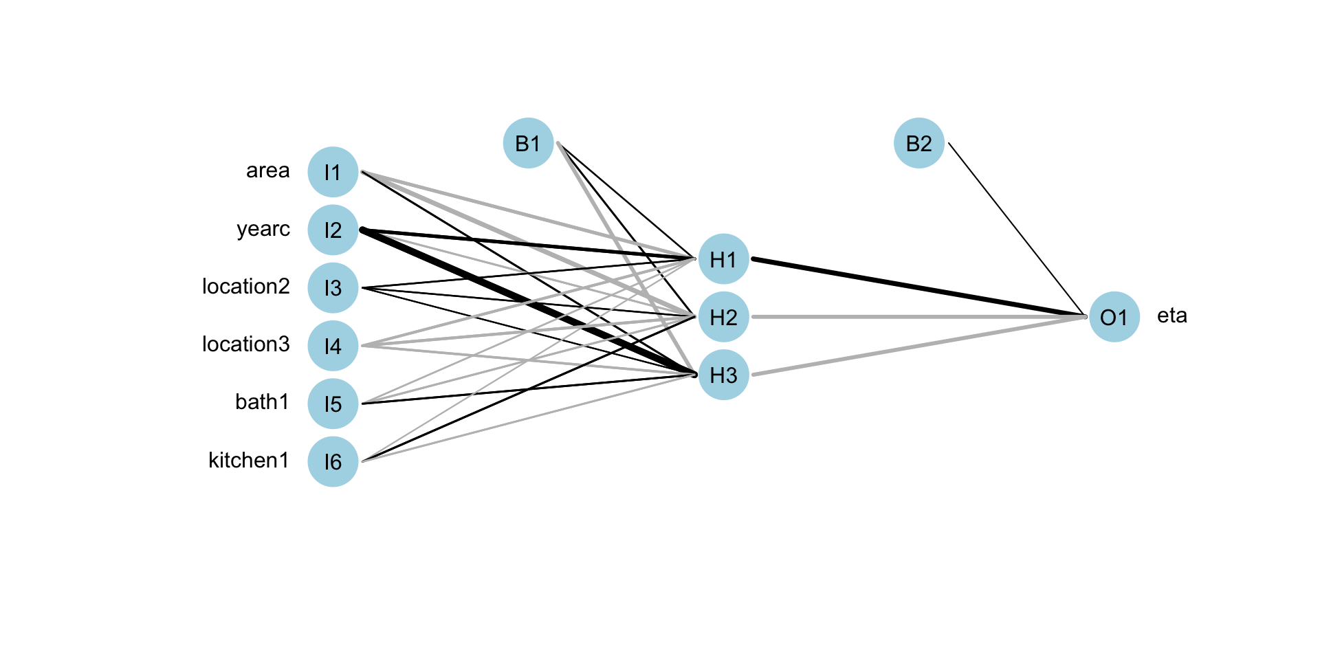
Neural Networks (fit)
f <- rent ~ n(~area+yearc+location+bath+kitchen, size=10)|      n(~area+yearc+location+bath+kitchen, size=3)
mneural <- gamlss2(f,family=BCTo, data=da)
GAMLSS-RS iteration 1: Global Deviance = 38208.8675 eps = 0.289873
GAMLSS-RS iteration 2: Global Deviance = 38178.0402 eps = 0.000806
GAMLSS-RS iteration 3: Global Deviance = 38177.034 eps = 0.000026
GAMLSS-RS iteration 4: Global Deviance = 38176.766 eps = 0.000007 AIC df
madditive 38196.95 32.2364
mlinear 38292.62 19.0000
mneural 38396.77 110.0000
mregtree 38754.64 30.0000Neural Networks (plot)
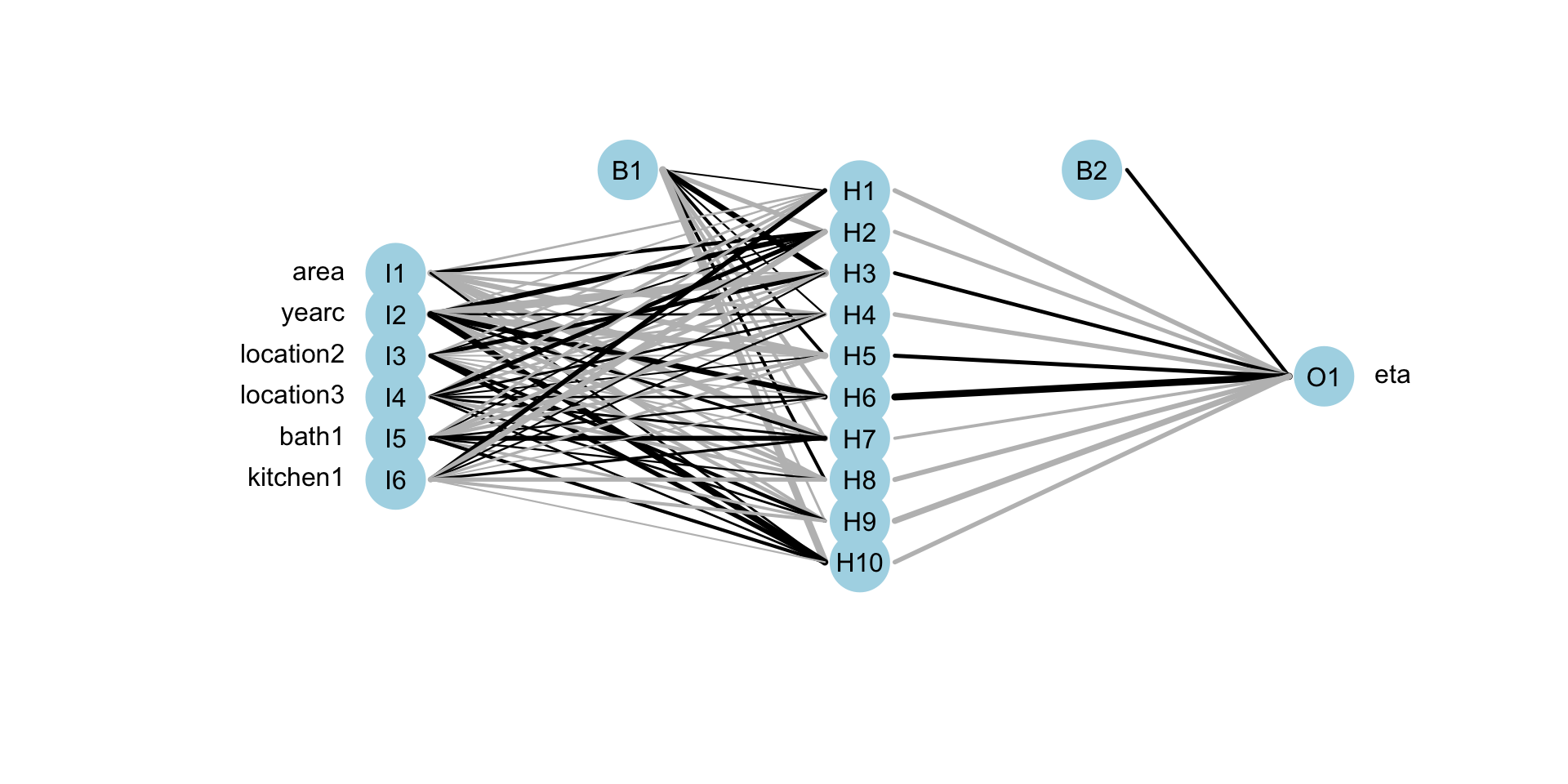
Neural Networks (plot)
random forest
f <- rent ~ cf(~area+yearc+location+bath+kitchen)|    cf(~area+yearc+location+bath+kitchen)
mcf <- gamlss2(f,family=BCTo, data=da)
GAMLSS-RS iteration 1: Global Deviance = 38465.948 eps = 0.285095
GAMLSS-RS iteration 2: Global Deviance = 38295.835 eps = 0.004422
GAMLSS-RS iteration 3: Global Deviance = 38289.9702 eps = 0.000153
GAMLSS-RS iteration 4: Global Deviance = 38288.2421 eps = 0.000045
GAMLSS-RS iteration 5: Global Deviance = 38287.9638 eps = 0.000007 AIC df
madditive 38196.95 32.2364
mlinear 38292.62 19.0000
mneural 38396.77 110.0000
mcf 38695.96 204.0000
mregtree 38754.64 30.0000LASSO-RIDGE
there is function
ri()ingamlssusing P-splinesthere is also package
gamlss.lassoforgamlssconnecting with packageglmnetbut LASSO is non implemented for
gamlss2yet
Principal Componet Regression
functions
pc()andpcr()ingamlss.foreachpackage forgamlssPCR is non implemented for
gamlss2yet
summary
| ML Models | coef. s.e. | stand. of x’s | algo. stab., speed, conv. | non-linear terms | inter- actions | data type | auto sele-ction | interpre- tation |
|---|---|---|---|---|---|---|---|---|
| linear | yes | no | yes, fast, v.good | poly | declare | \(n>r\) | no | v. easy |
| additive | no | no | yes, slow, good | smooth | declare | \(n>r\) | no | easy |
| RT | no | no | no, slow, bad | trees | auto | \(n>r\)?? | yes | easy |
summary (continue)
| ML Models | coef. s.e. | stand. of x’s | algo. stab., speed, conv. | non-linear terms | inter- actions | data type | auto sele-ction | interpre- tation |
|---|---|---|---|---|---|---|---|---|
| NN | no | 0 to 1 | no, \(\,\,\) ok, \(\,\,\) ok | auto | auto | both? | yes | v. hard |
| RF | no | no | no, slow, slow | YES | no | both | auto | hard |
| LASSO | no | yes | yes, fast, good | poly | declare | both | auto | easy |
summary (continue)
| ML Models | coef. s.e. | stand. of x’s | algo. stab., speed, conv. | non-linear terms | inter- actions | data type | auto sele-ction | interpre- tation |
|---|---|---|---|---|---|---|---|---|
| Boost | no | no | yes, fast, good | smooth trees | declare | \(n<<r\) | yes | easy |
| MCMC | yes | no | good, ok, \(\,\,\) ok | smooth | declare | \(n>r\) | no | easy |
| PCR | yes | yes | yes, fast, good | poly | declare | both | auto | hard |
end
 The Books
![]()
www.gamlss.com