Diagnostics and ggplots

Mikis Stasinopoulos
Bob Rigby
Fernanda De Bastiani
Gillian Heller
Niki Umlauf

Graphical Diagnostic tools

  • individual variable/data information

  • models dianostics

    • within model

    • between models

data and models

library(gamlss2)
library(gamlss.ggplots)
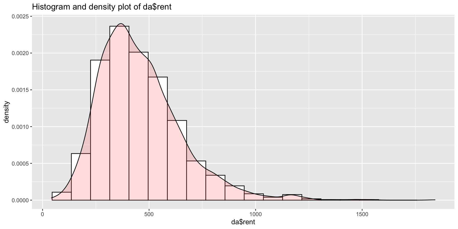
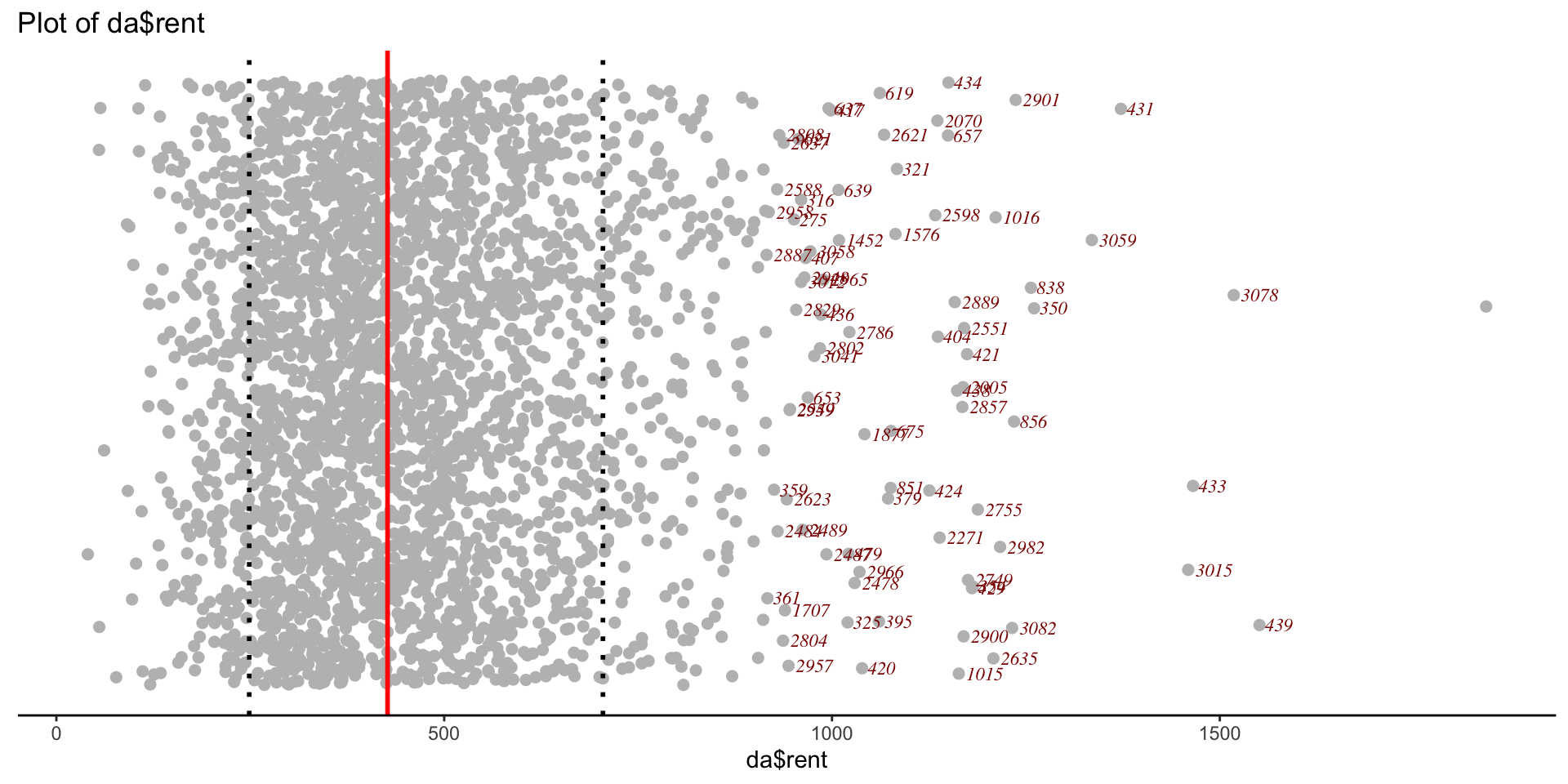
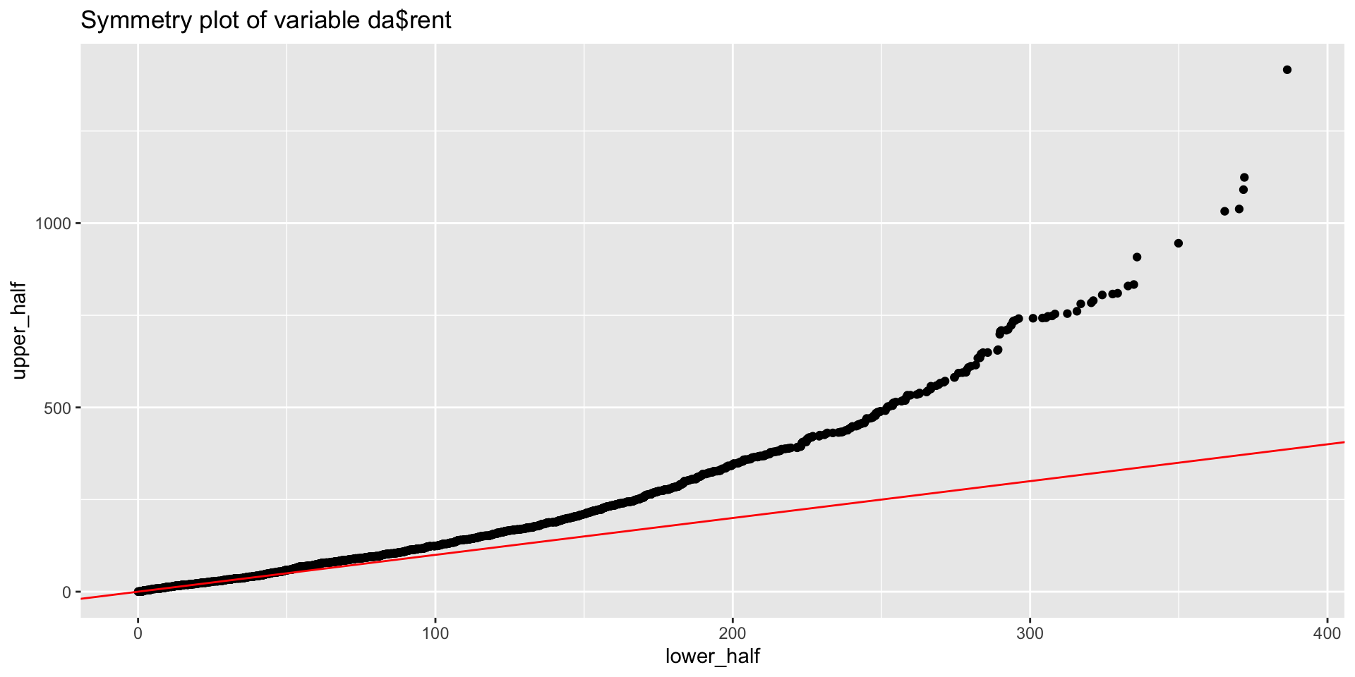
da <- rent99[,-c(2,9)]
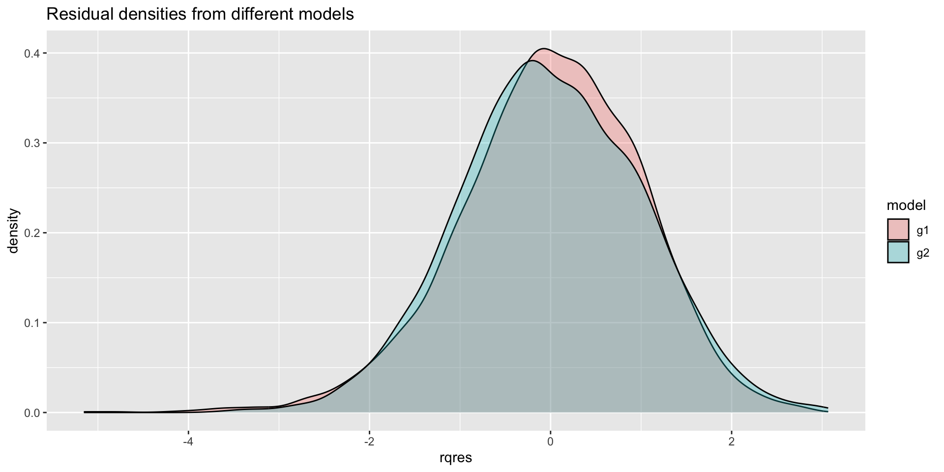
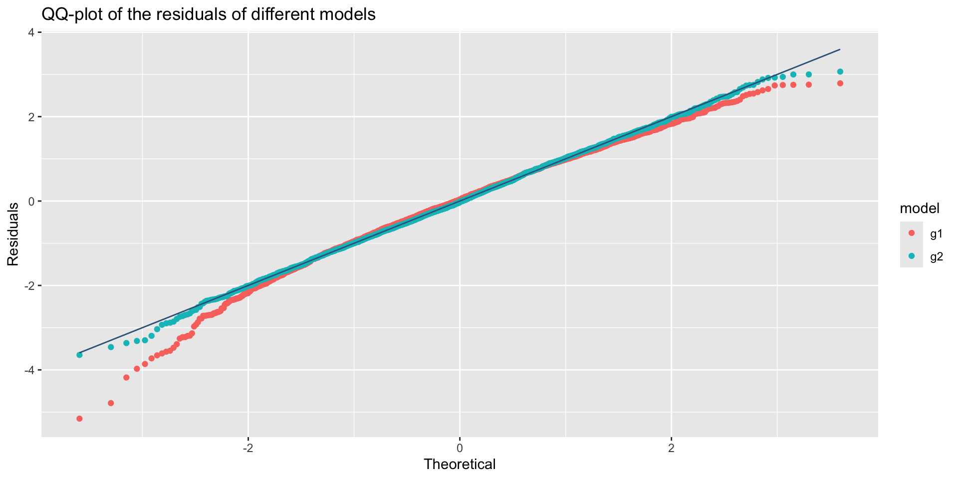
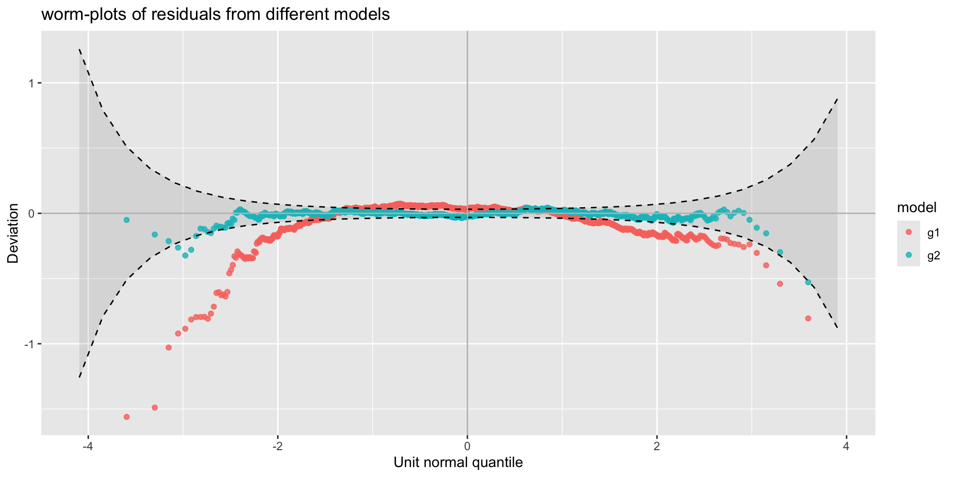
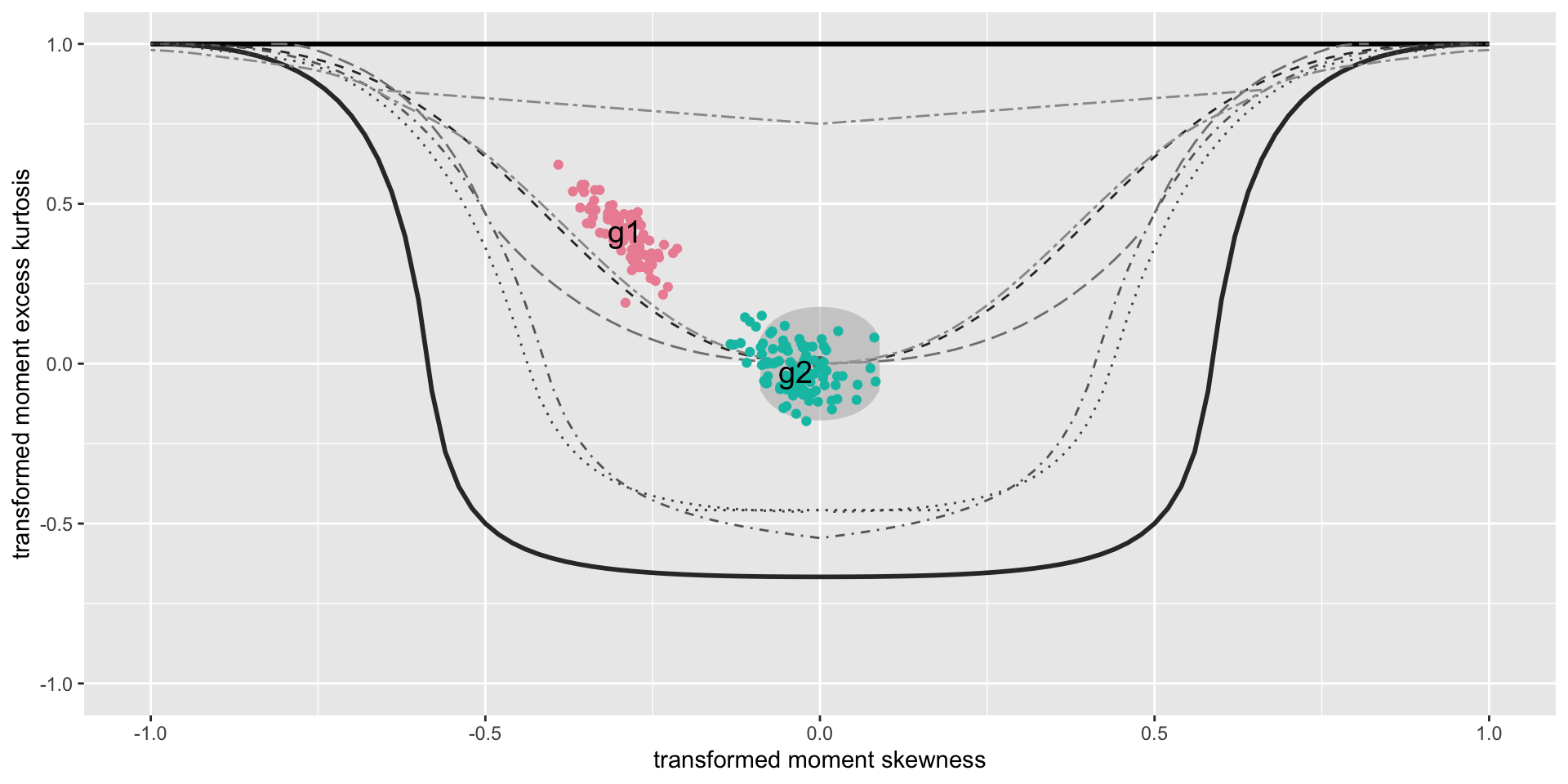
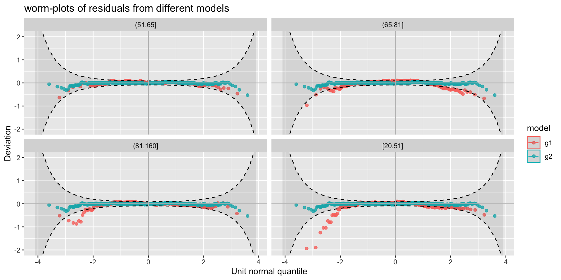
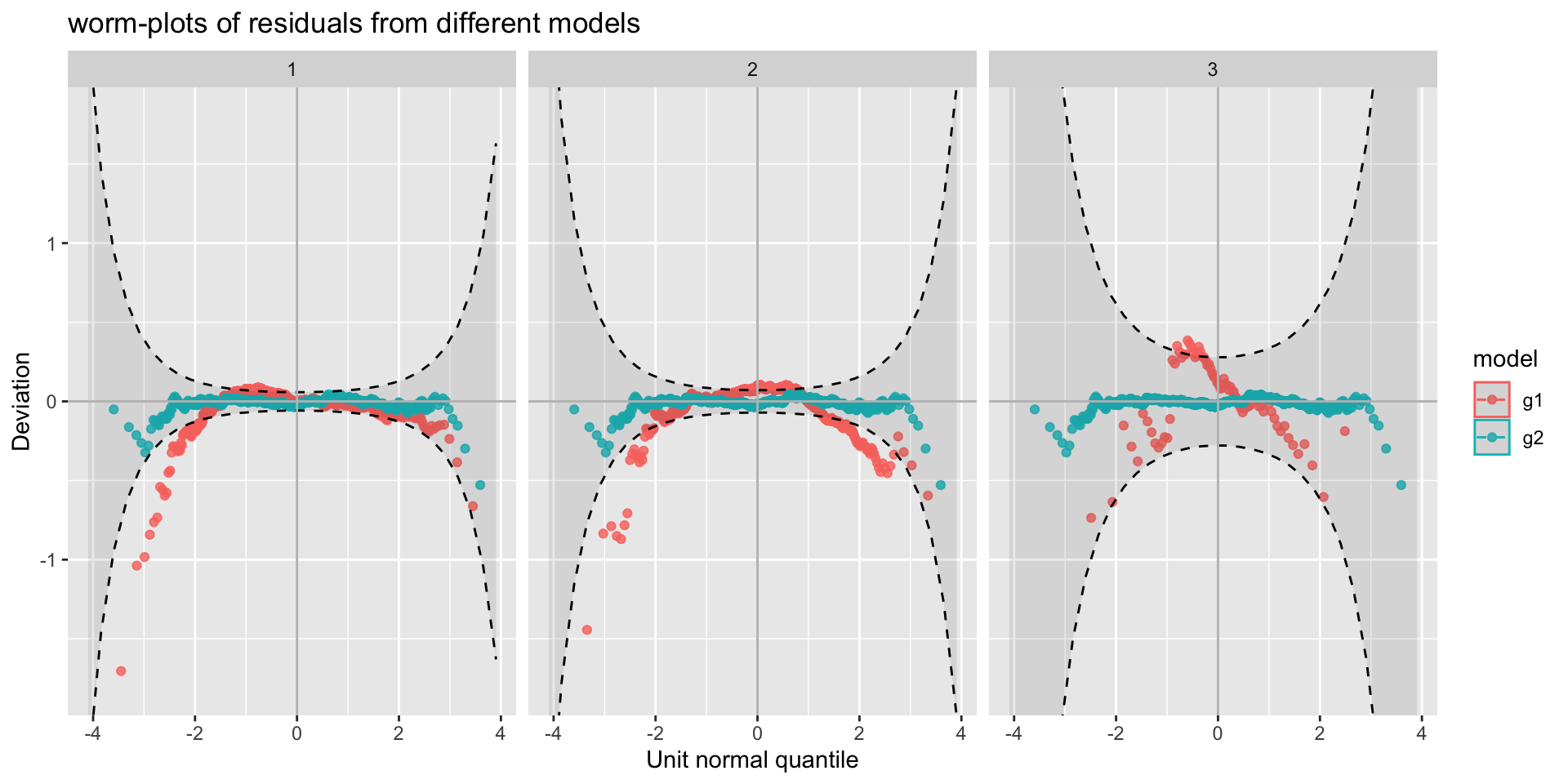
g1 <- gamlss2(rent~s(area)+s(yearc)+bath+location+kitchen+cheating|
s(area)+s(yearc)+bath+location+kitchen+cheating, data=da, family=GA )
GAMLSS-RS iteration  1: Global Deviance = 38249.9521 eps = 0.129707     
GAMLSS-RS iteration  2: Global Deviance = 38205.9938 eps = 0.001149     
GAMLSS-RS iteration  3: Global Deviance = 38205.9065 eps = 0.000002     
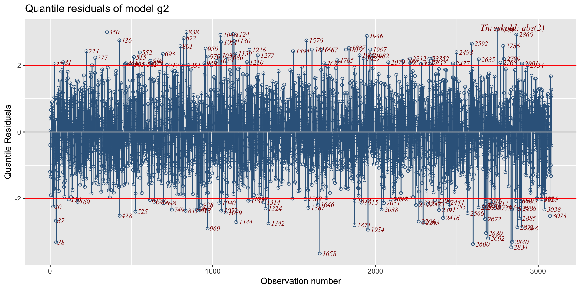
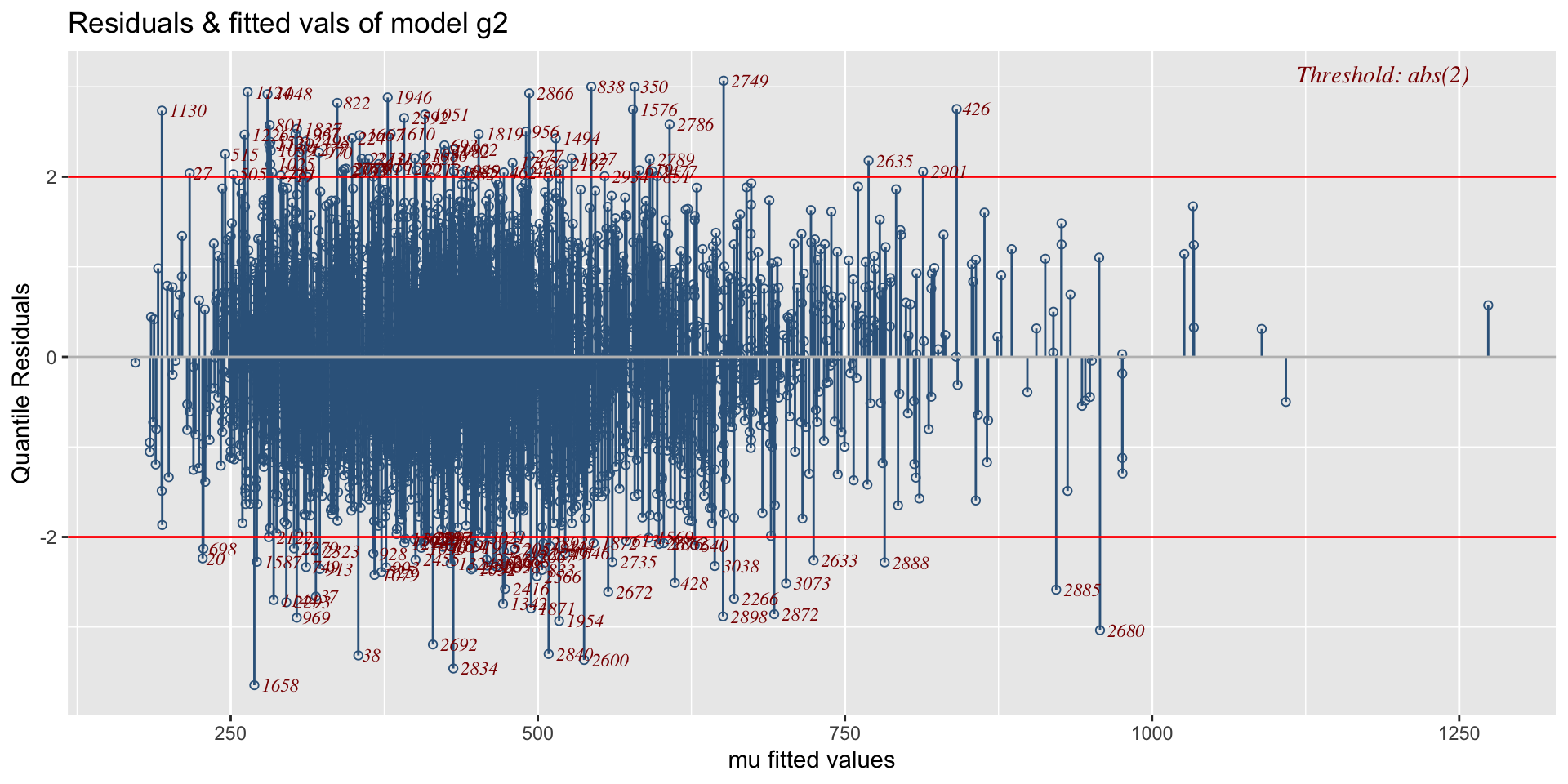
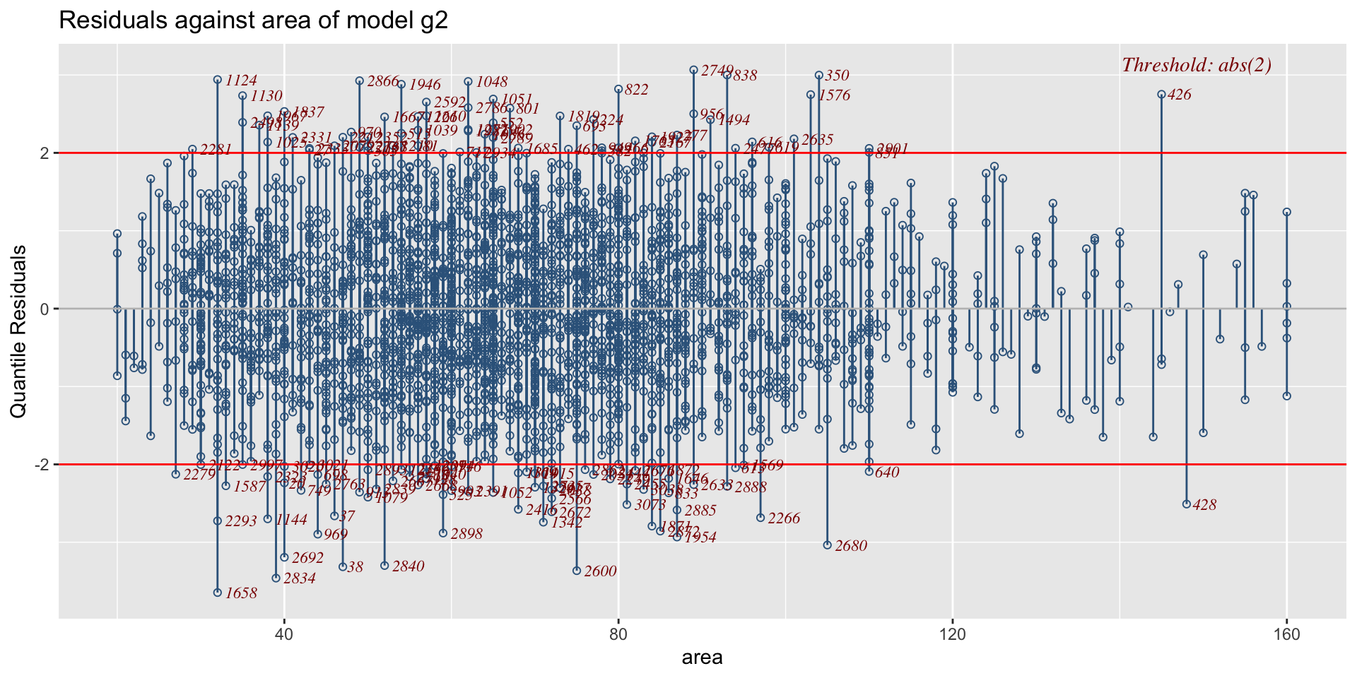
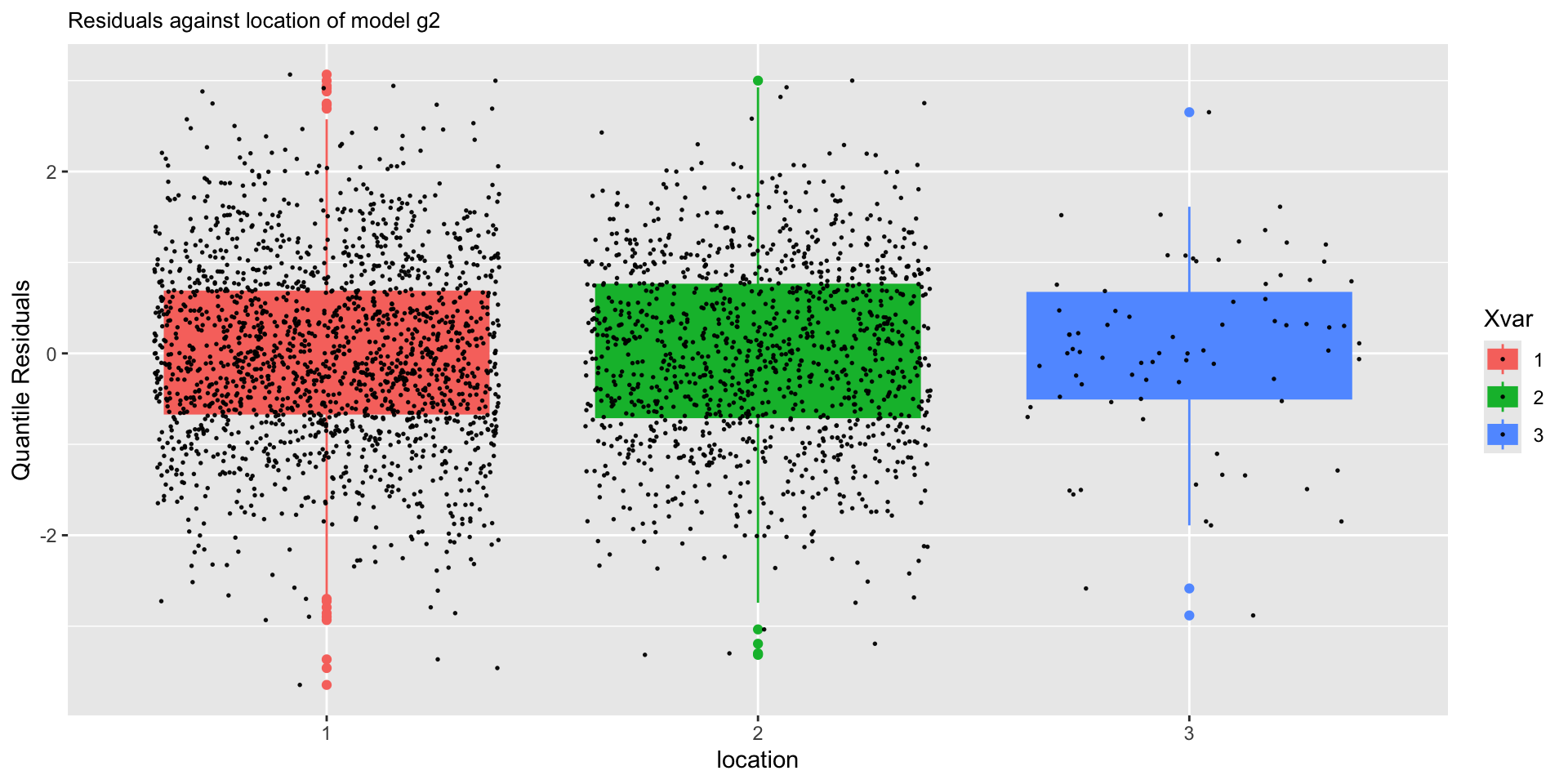
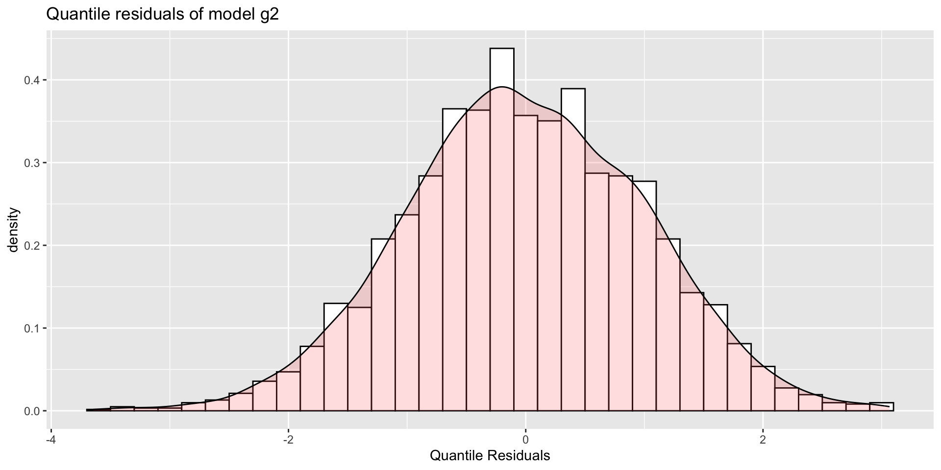
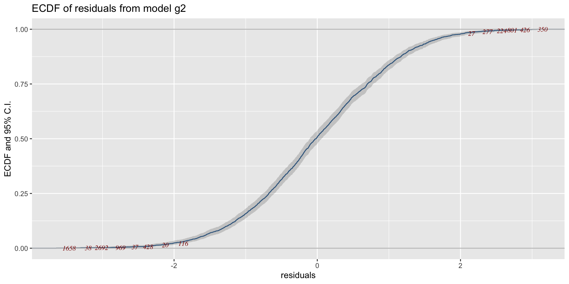
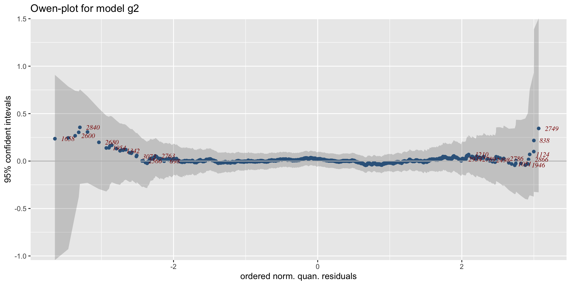
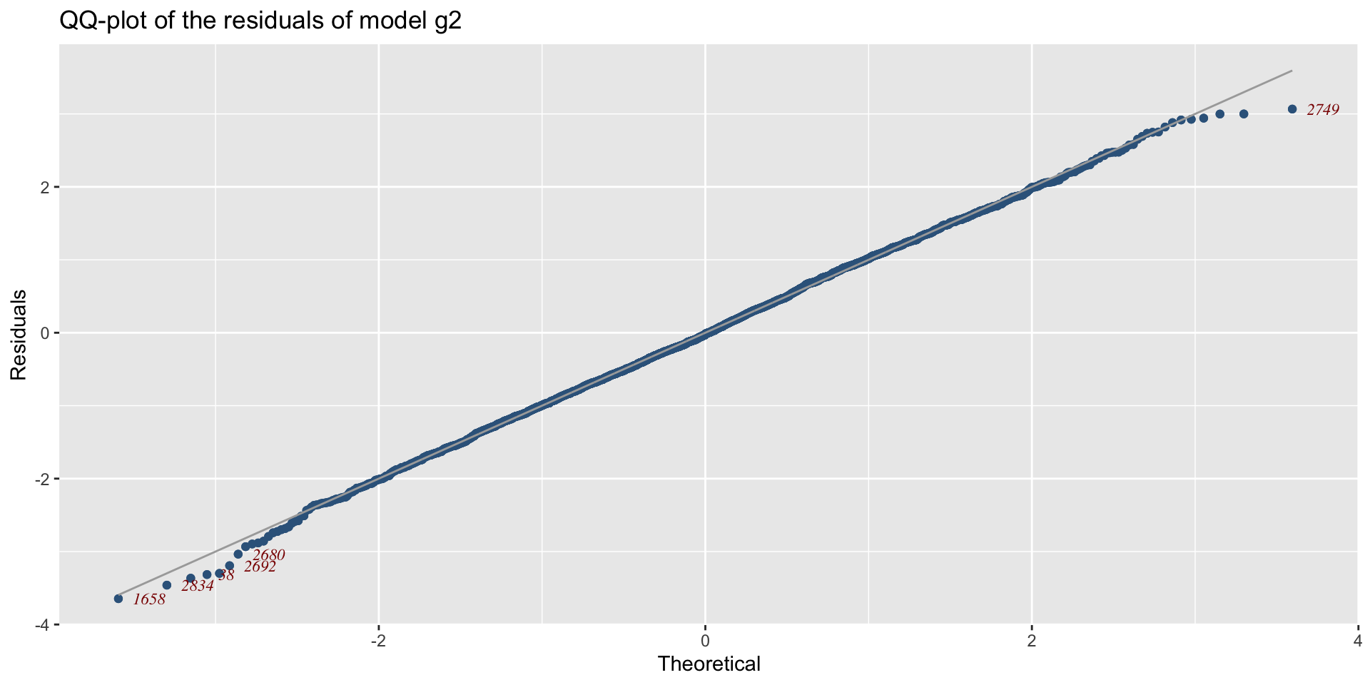
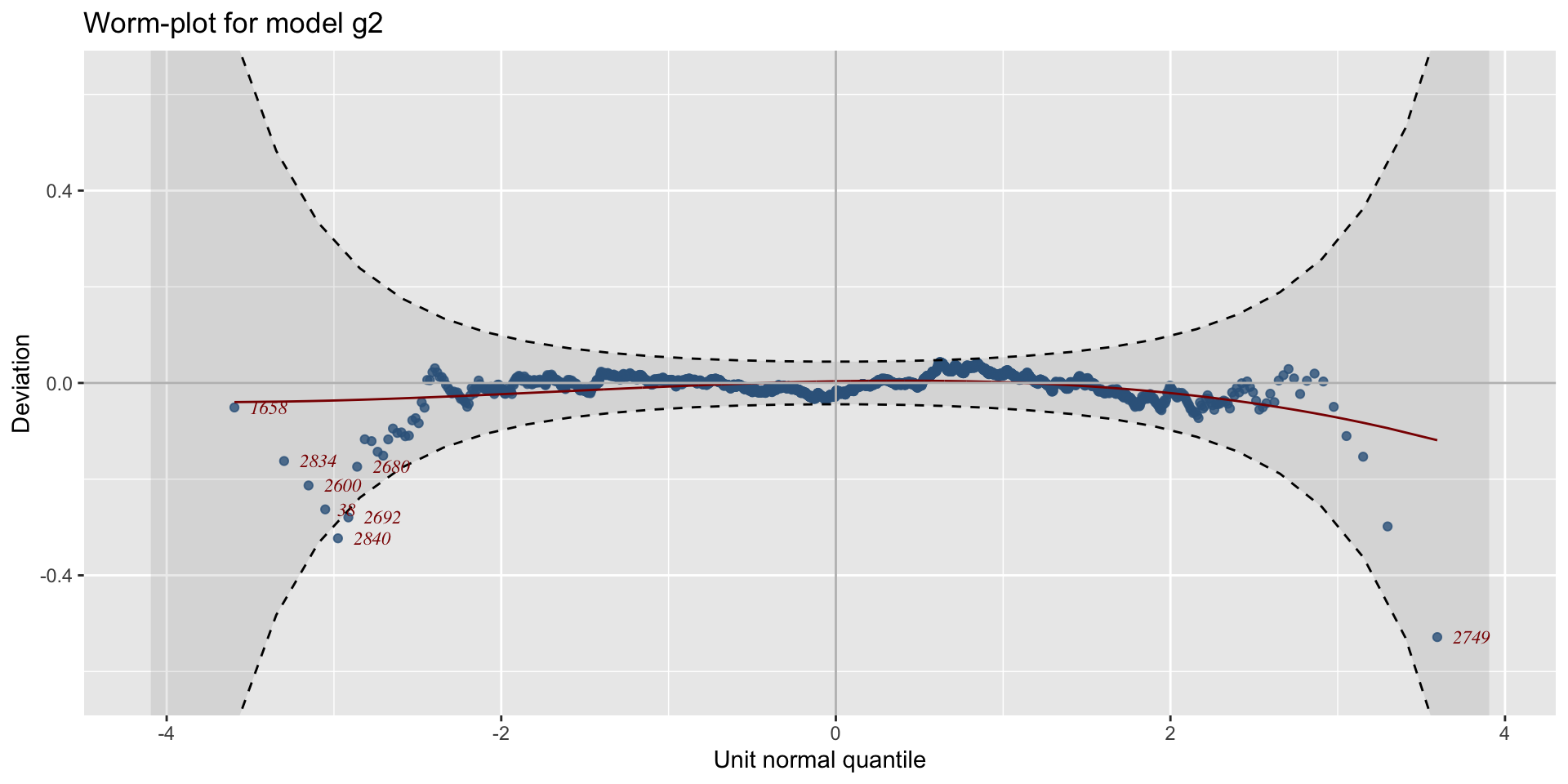
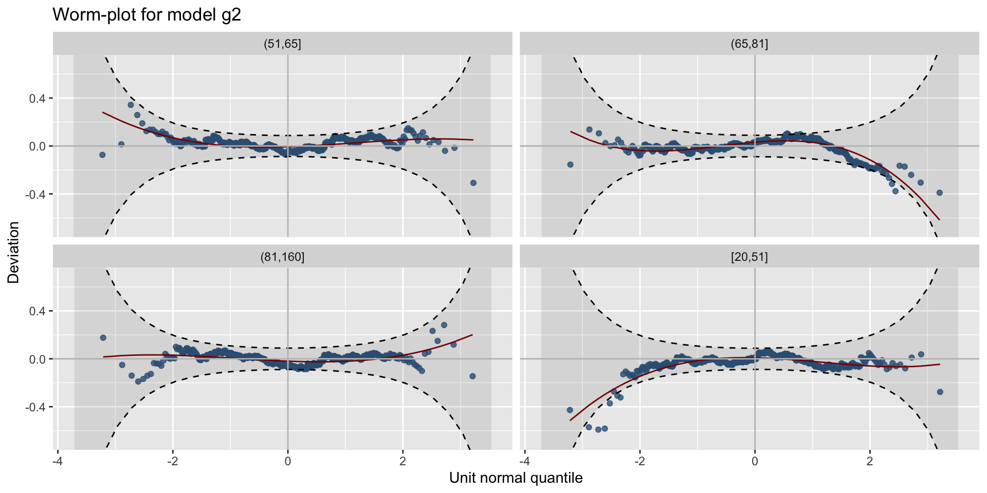
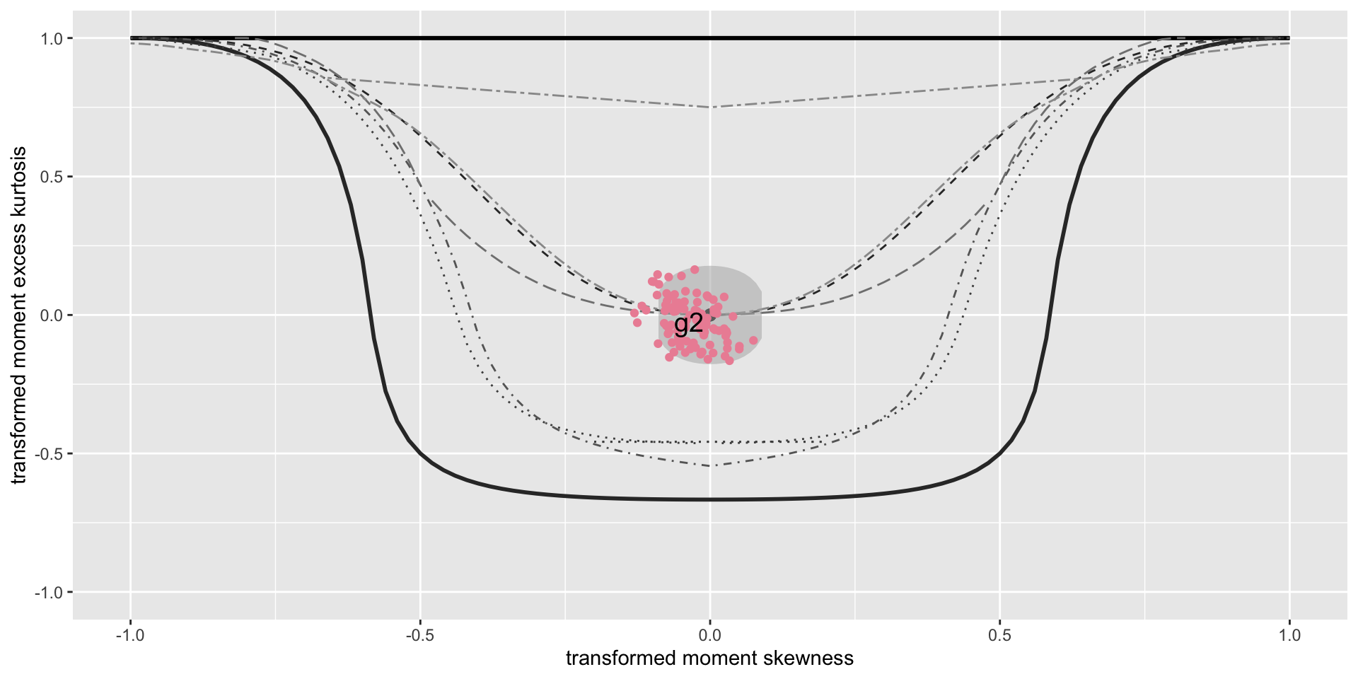
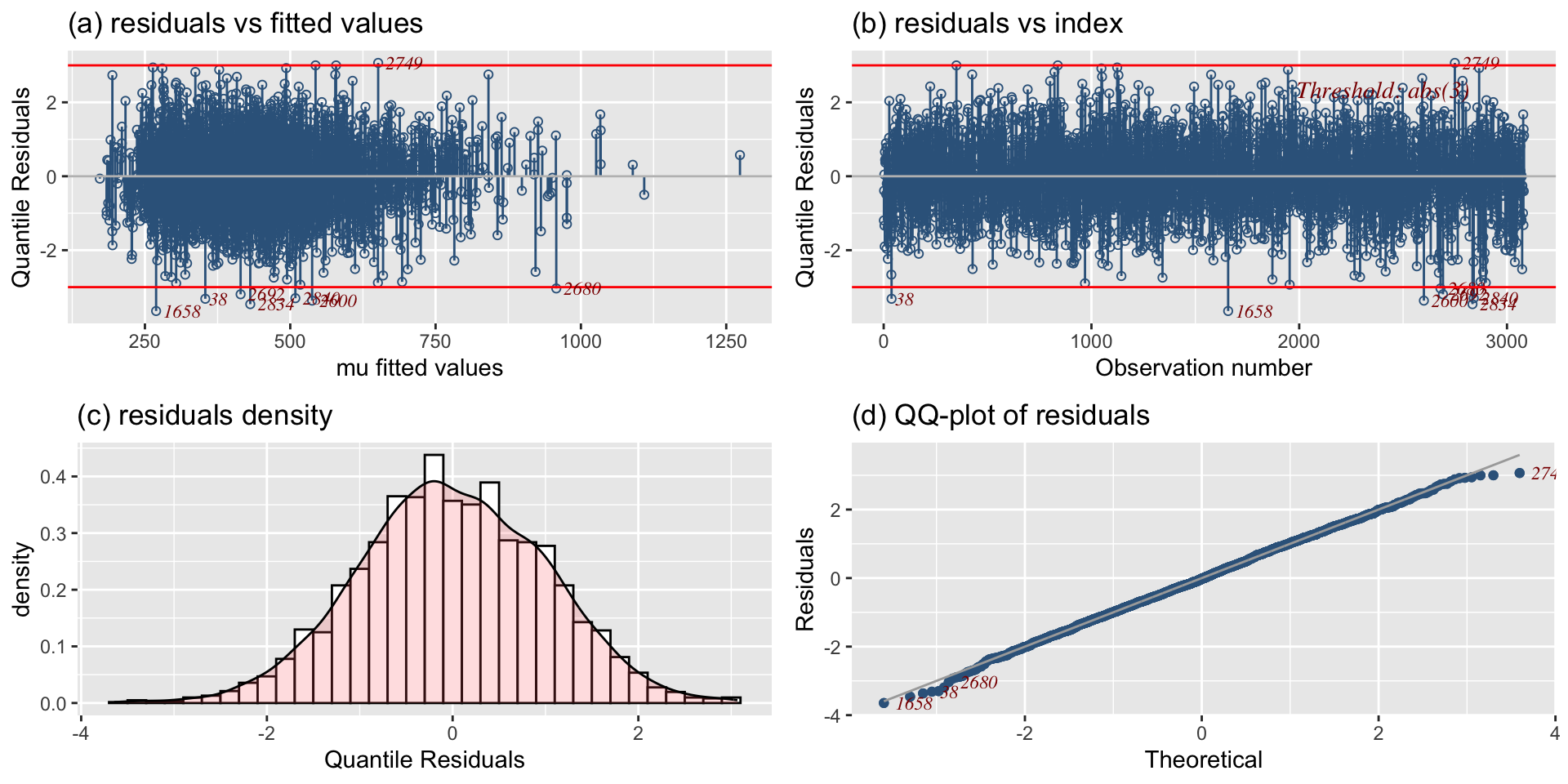
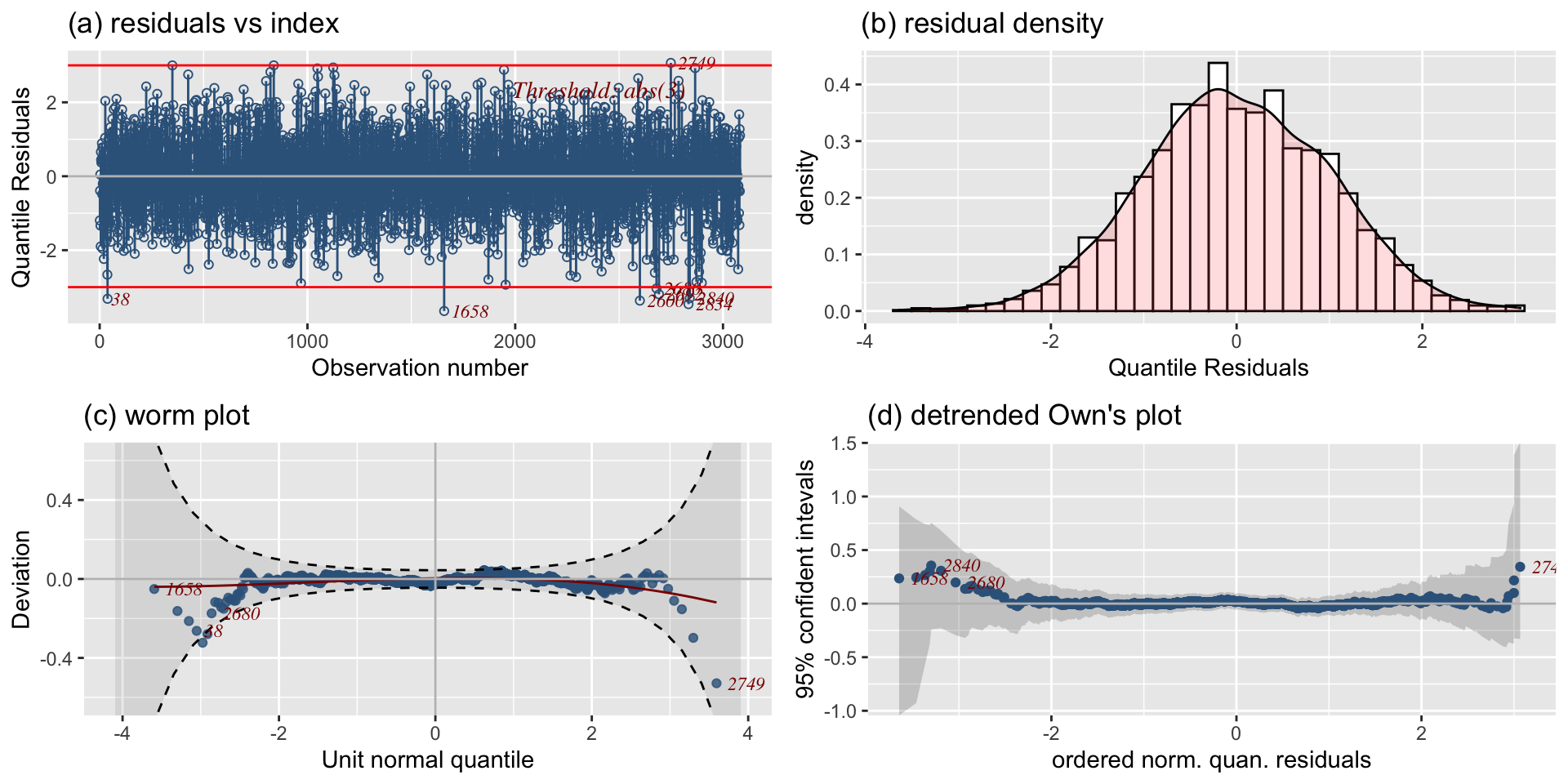
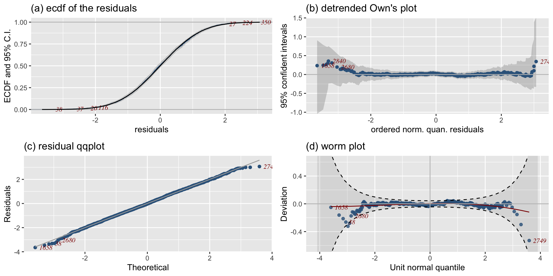
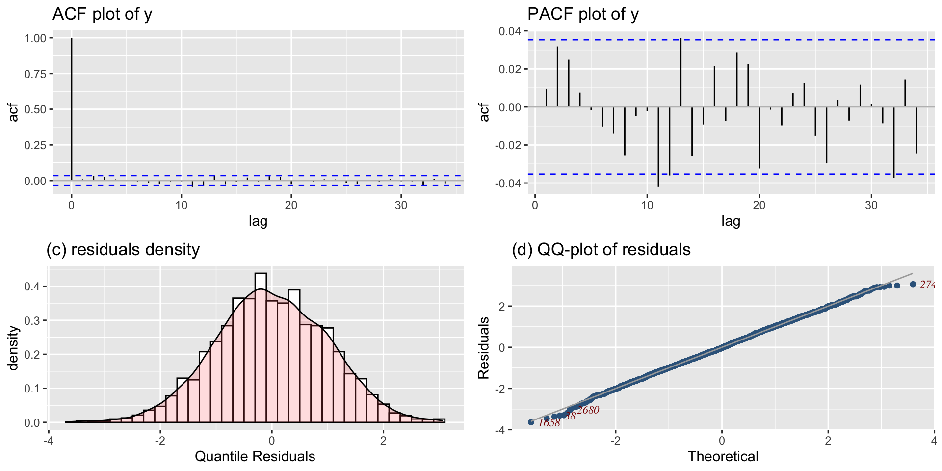
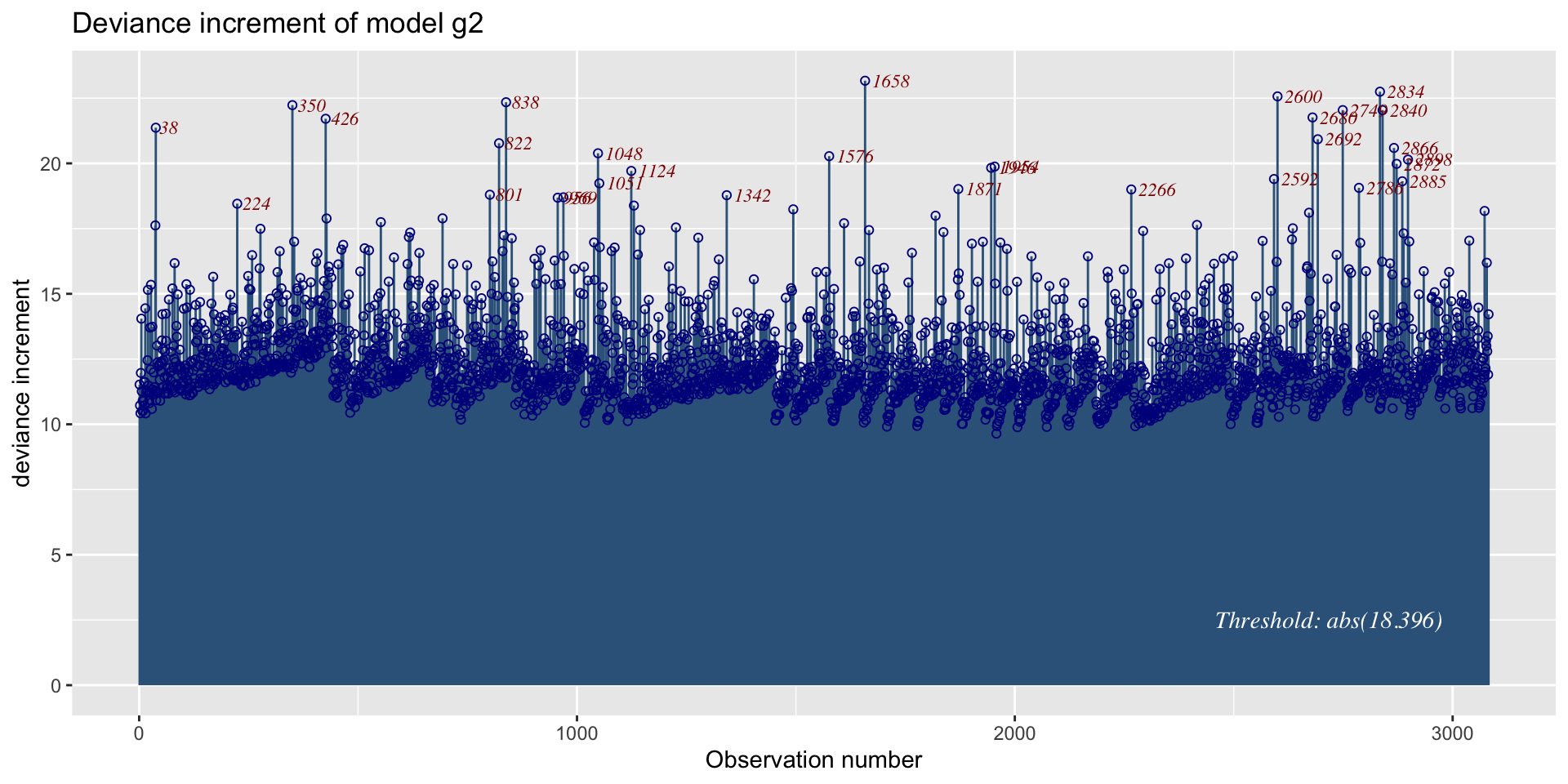
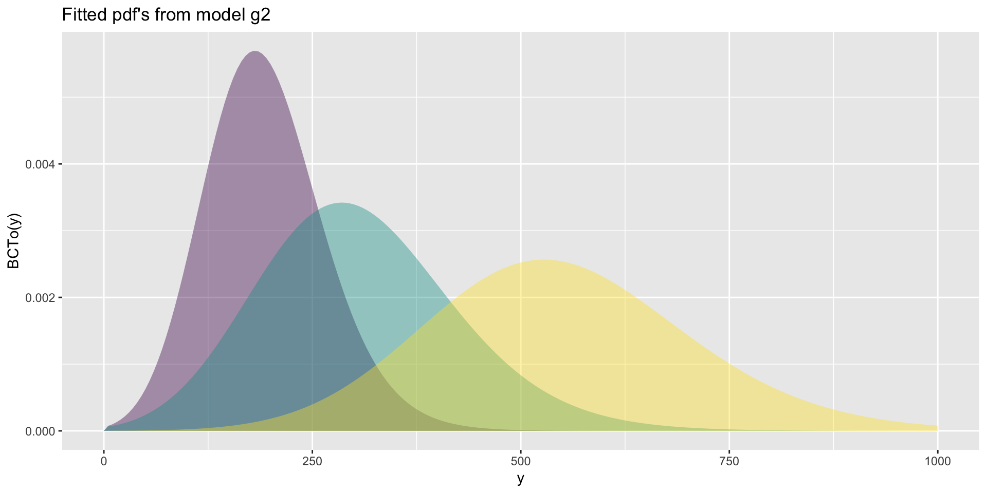
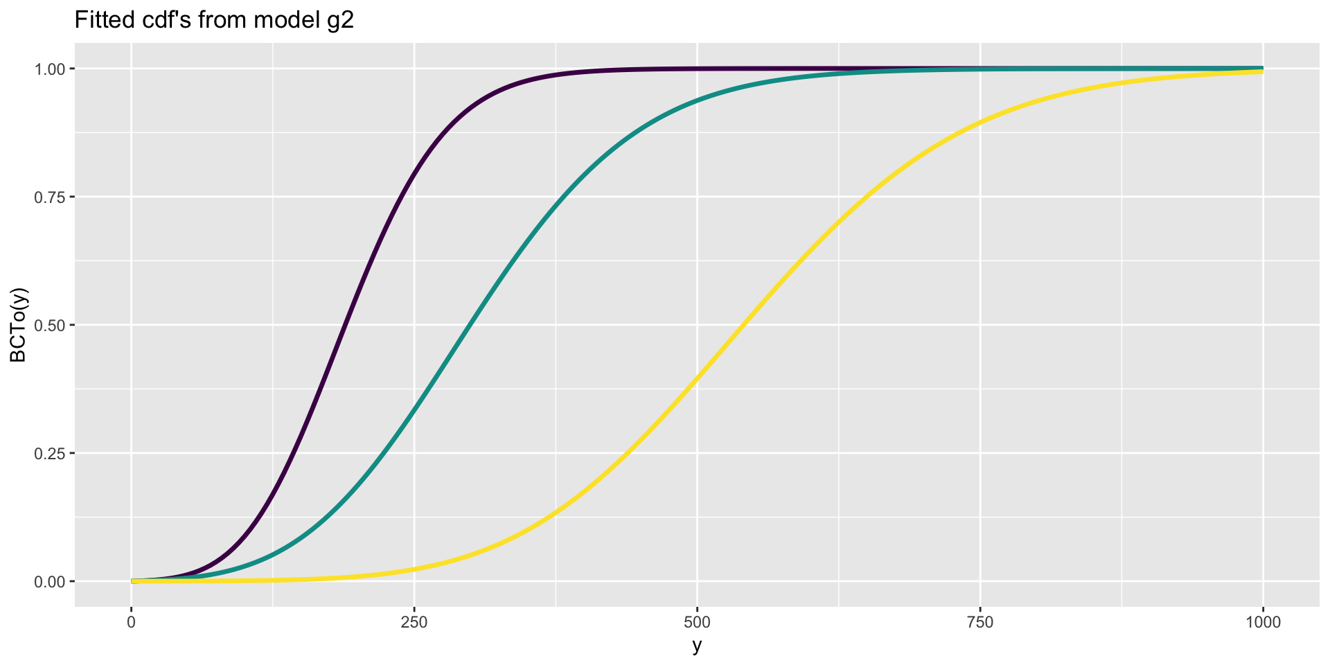
g2 <- gamlss2(rent~s(area)+s(yearc)+bath+location+kitchen+cheating|
s(area)+s(yearc)+bath+location+kitchen+cheating, data=da, family=BCTo )
GAMLSS-RS iteration  1: Global Deviance = 38170.7368 eps = 0.290582     
GAMLSS-RS iteration  2: Global Deviance = 38135.3004 eps = 0.000928     
GAMLSS-RS iteration  3: Global Deviance = 38133.3037 eps = 0.000052     
GAMLSS-RS iteration  4: Global Deviance = 38132.6789 eps = 0.000016     
GAMLSS-RS iteration  5: Global Deviance = 38132.4637 eps = 0.000005     
gamlss2::GAIC(g1,g2)
        AIC       df
g2 38196.95 32.24370
g1 38267.22 30.65513

individual variables

y_hist()

y_hist(da$rent)

y_dots()

y_dots(da$rent)

y_symmetry()

y_symmetry(da$rent)

y_acf() time series

y_acf(da$rent)

y_pacf() time series

y_pacf(da$rent)

moment_bucket()

moment_bucket(da$rent)

data_plot()

library(gamlss.prepdata)
data_plot(da)
only 100 % of data are ploted, 
that is, 3082 observations. 

data_xyplot()

library(gamlss.prepdata)
data_xyplot(da, response=rent)
100 % of data are ploted, 
that is, 3082 observations. 

model diagnostics

within model

residuals against index

resid_index(g2)

residuals against \(\mu\)

resid_mu(g2)

residuals against quantile value

resid_quantile(g2)

residuals against x-var (cont.)

resid_xvar(g2, xvar=area)

residuals against x-var (factor)

resid_xvar(g2, xvar=location)

residual density

resid_density(g2)

ECDF residual plot

resid_ecdf(g2)

detrended ECDF plot

resid_dtop(g2)

both ECDF

(a) ecdf
(b) Own’s detrened plot
Figure 1: the ECDF and DTOP give the same information

QQ-plot

resid_qqplot(g2)

worm plot

resid_wp(g2)

QQ and worm plots

(a) QQ-plot
(b) worm-plot
Figure 2: QQ and worm plots (same infrmation)

worm plot for x-var

resid_wp_wrap(g2, xvar=rent99$area)

Bucket plots

resid_plots() standard

resid_plots(g2)

resid_plots() new

resid_plots(g2, theme="new")

resid_plots() ECDF

resid_plots(g2, theme="ecdf")

resid_plots() TS

resid_plots(g2, theme="ts")

deviance increment

fitted_devianceIncr(g2)

fitted distributions (pdf)

fitted_pdf(g2, c(1, 100, 1000), from=0, to=1000)

fitted distributions (cdf)

fitted_cdf(g2, c(1, 100, 1000), from=0, to=1000)

between models diagnostics

model density

Figure 3: The model density estimates of the residuals

model QQ-plots

(a) QQ-plots

model worm-plots

(a) worm plots

model bucket plot

(a) bucket plot

model wp wrap

Figure 7: Worm plots for different fitted models at different values of the continuous variable area

model wp wrap (continue)

Figure 8: Worm plots for different fitted models at different levels of the factor location

model deviance increment difference

Practical 5

END

back to the index

The Books