| R | Fl | A | B | H | L | loc |
|---|---|---|---|---|---|---|
| 693.3 | 50 | 1972 | 0 | 0 | 0 | 2 |
| 422.0 | 54 | 1972 | 0 | 0 | 0 | 2 |
| 736.6 | 70 | 1972 | 0 | 0 | 0 | 2 |
| 732.2 | 50 | 1972 | 0 | 0 | 0 | 2 |
| 1295.1 | 55 | 1893 | 0 | 0 | 0 | 2 |
| 1195.9 | 59 | 1893 | 0 | 0 | 0 | 2 |
The R software
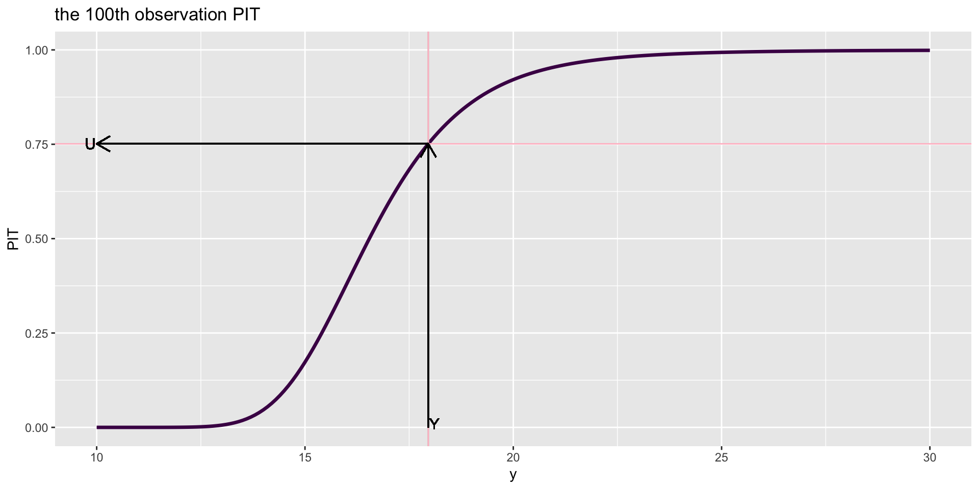
PIT
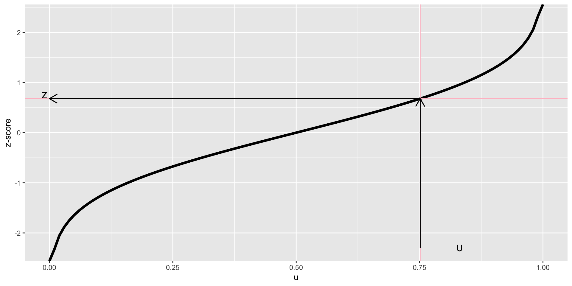
z-scores
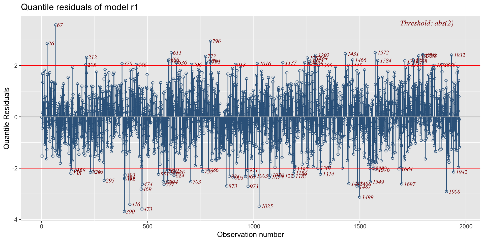
residual plots agaist index
against continuous x-variables

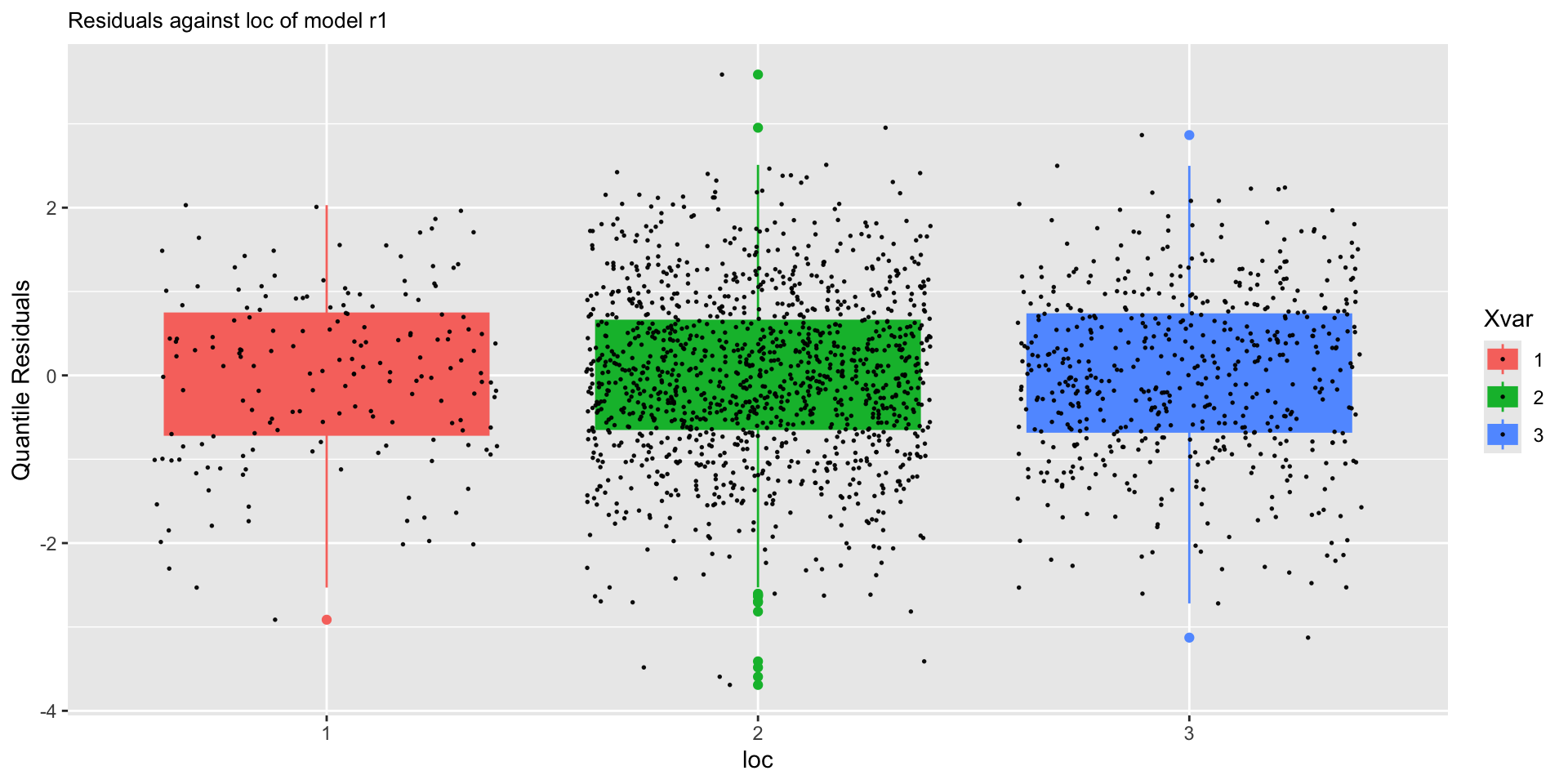
against factor x-variables
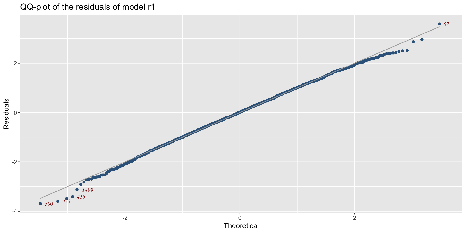
QQ-plots
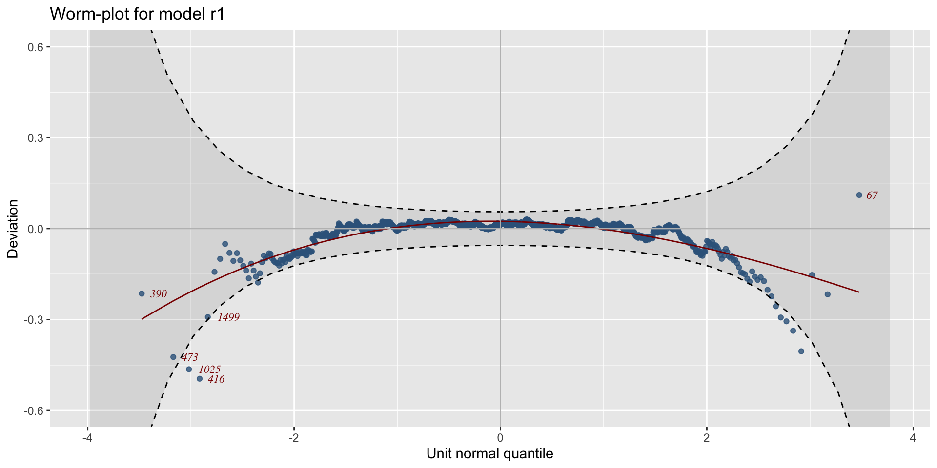
worm plots
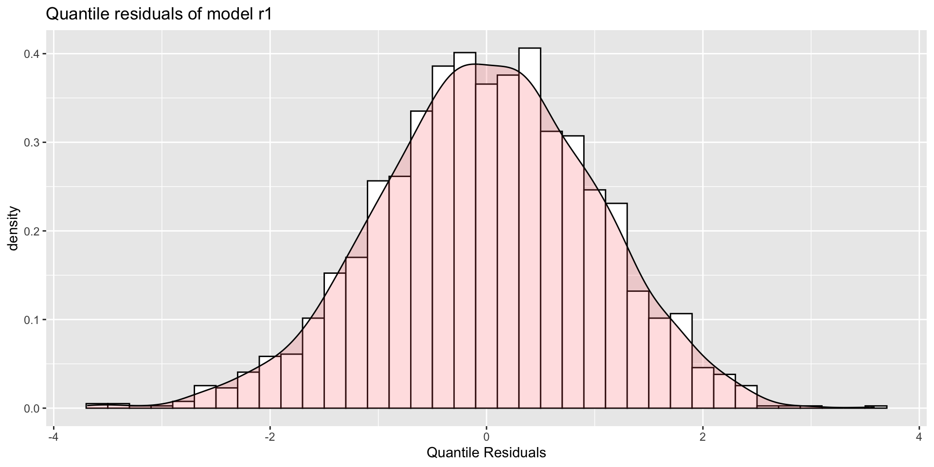
density plots
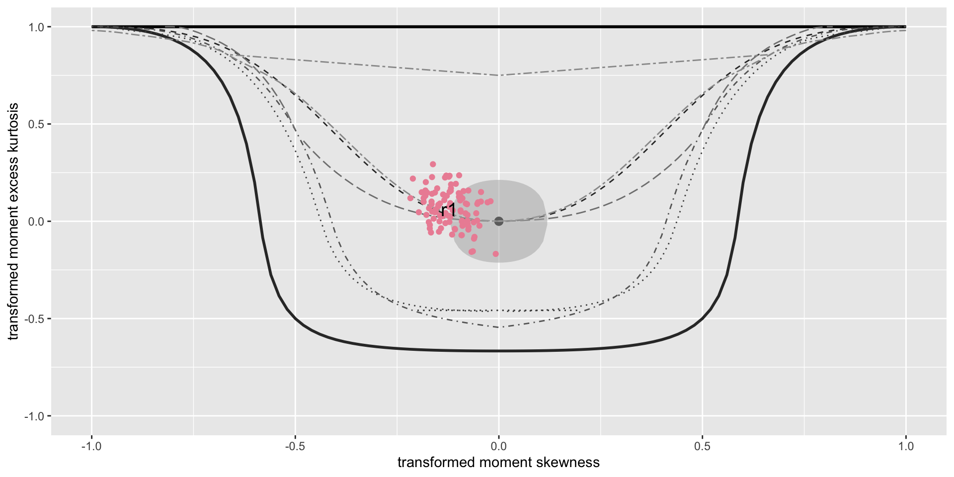
bucket plots
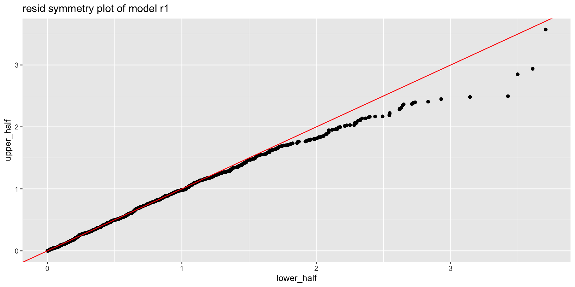
symmetry plots
ecdf plot

detrended ecdf plot
all in one plots
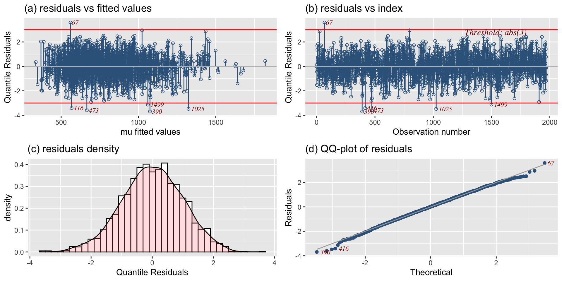
all in one plots (standard)

end

 The Books
![]()