Mixed Distributions

Mikis Stasinopoulos

Bob Rigby

Fernanda De Bastiani

Gillian Heller

Niki Umlauf

introduction

A mixed distribution is special case of a finite mixture distribution
it has two components: a continuous distribution and a discrete distribution
it is a continuous distribution where the range of $Y$ also includes discrete values with non-zero probabilities.

Types

Zero adjusted distributions on $[0, \infty]$
inflated distributions on $[0,1]$

– $[0,1)$ inflated at zero

– $(0,1]$ inflated at one

– $[0,1]$ inflated at zero and one

Zero adjusted distributions

explicit: (they exist in gamlss.dist package)
impicit (they can be generated generated using the package gamlss.inf)

Explicit mixed dist (con.)

name	gamlss	range	parameter-links
beta inf.	`BEINF0`	$[0, 1)$	logit , logit , log , -
beta-inf.	`BEOI`	$[0 , 1)$	logit , log , logit , -
beta 1-inf.	`BEINF1`	$(0, 1]$	logit , logit , log , -
beta 1-inf.	`BEZI`	$(0, 1]$	logit, log, logit, -
beta 0 & 1 inf	`BEINF`	$[0, 1]$	logit, logit, log, log
gamma 0-adj.	`ZAGA`	$[0, \infty)$	log, log, logit, -
inv Gaussian 0-adj	`ZAIG`	$[0, \infty)$	log, log, logit, -

zero adjusted

\[\begin{split} f_Y(y)= \begin{cases} p & \mbox{if } y=0 \\ (1-p)f_{Y_1}(y) & \mbox{if } y>0\ . \end{cases} \label{E:MPFZAW} \end{split}\]

cdf \[\begin{equation} P(Y \leq y)= p + (1-p) P (Y_1 \leq y) \label{E:CDFZAW} \end{equation}\]

zero adjusted con.

example zero adjusted

library(gamlss.inf)
gen.Family(family="SST", type="log")

A  log  family of distributions from SST has been generated 
 and saved under the names:  
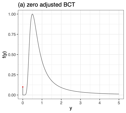
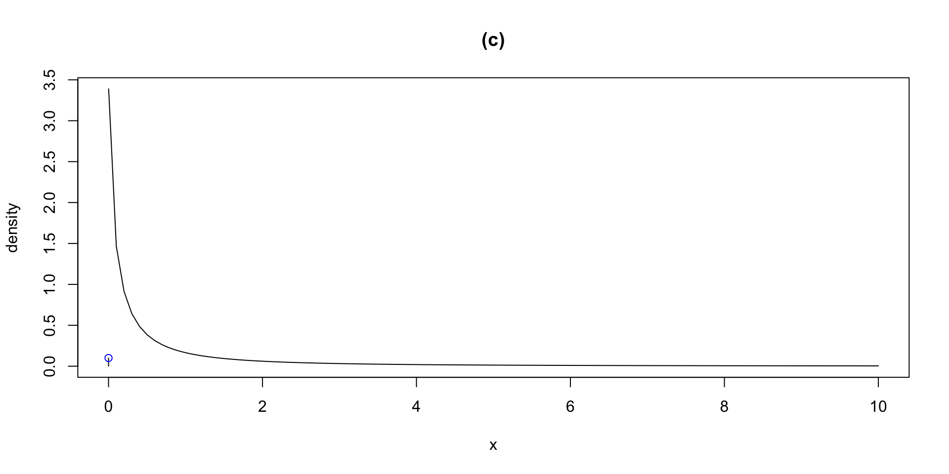
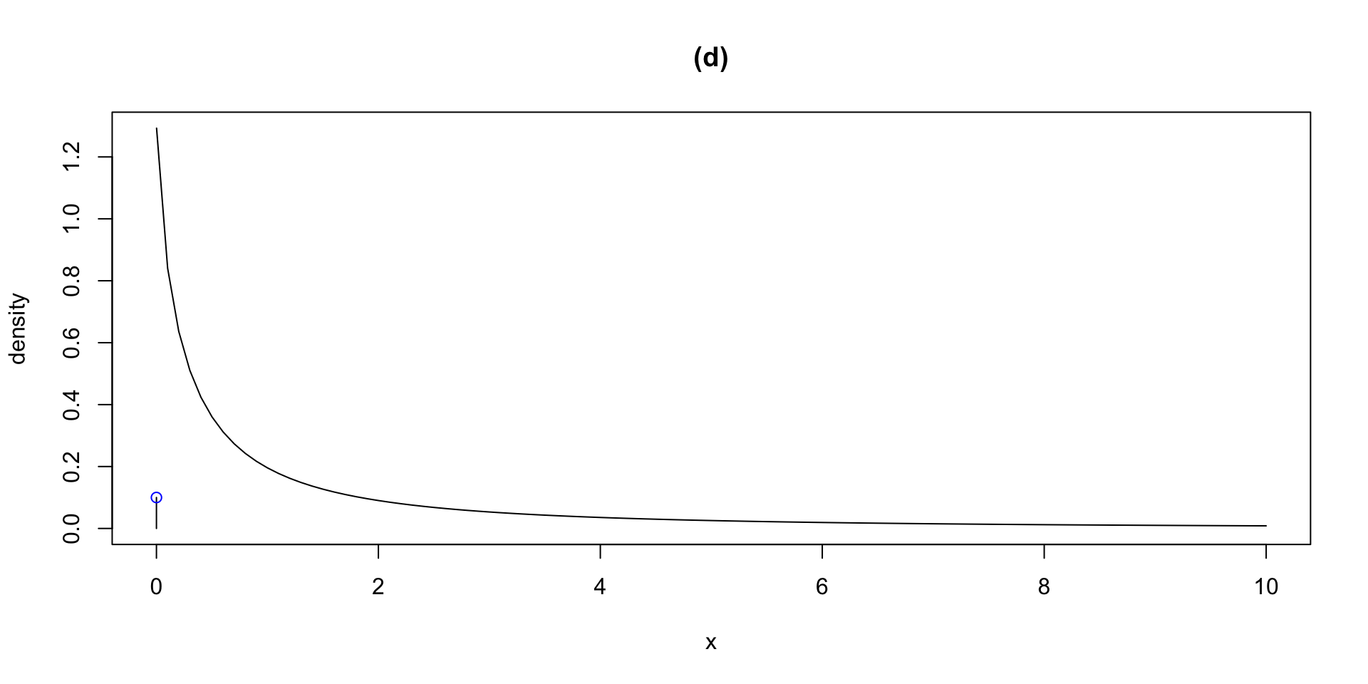
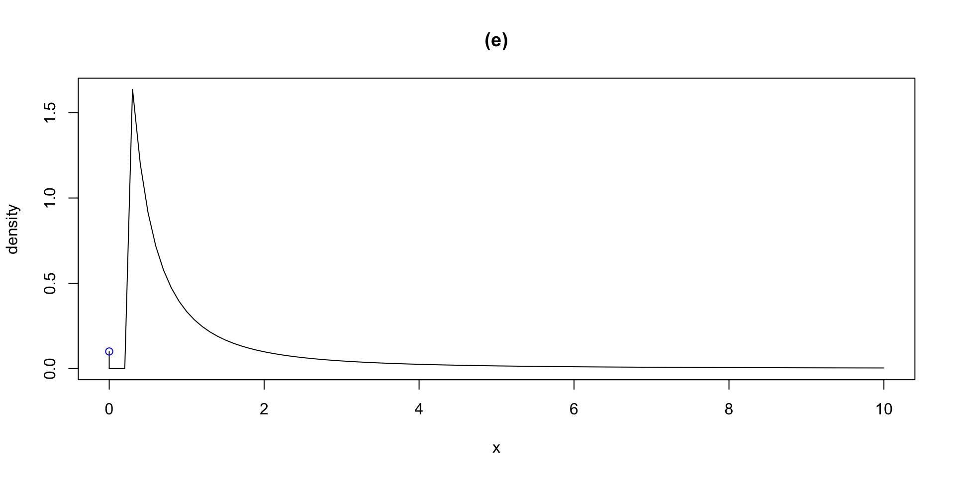
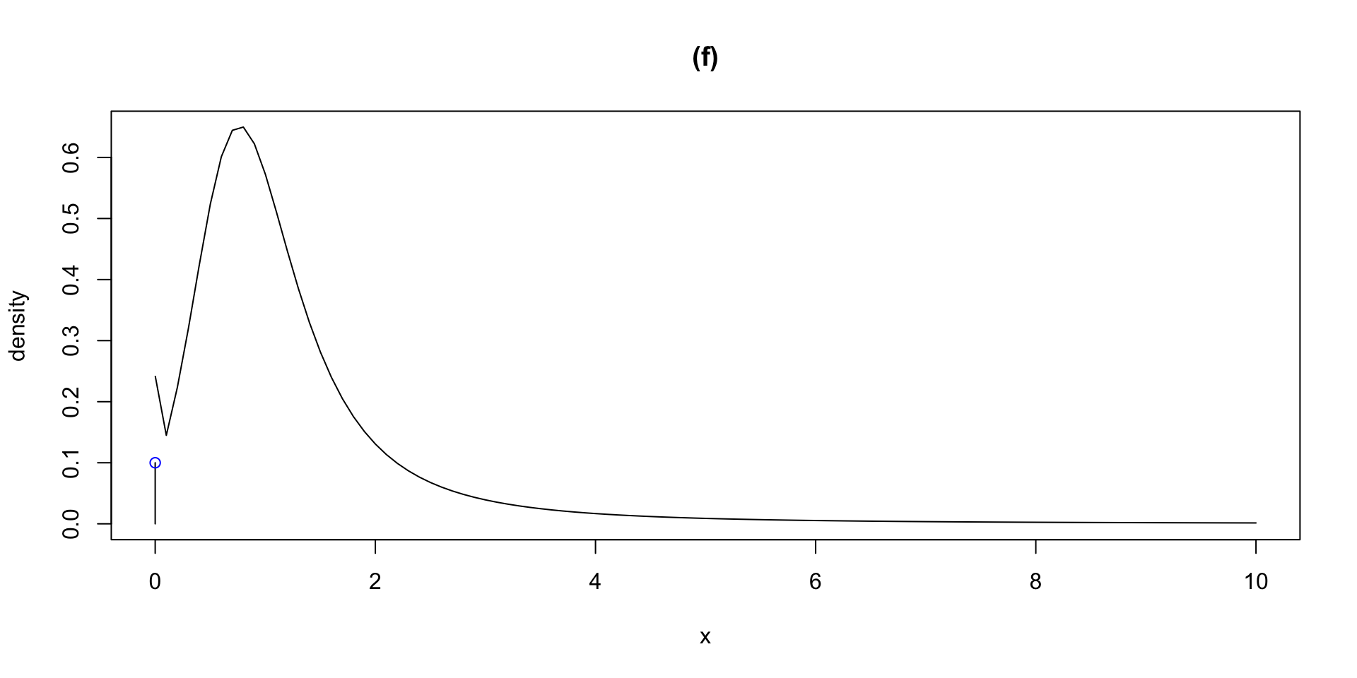
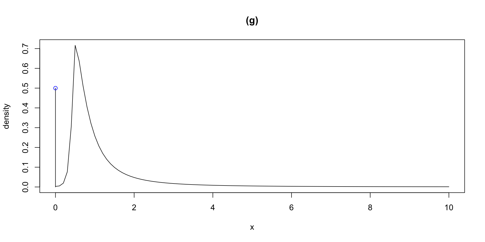
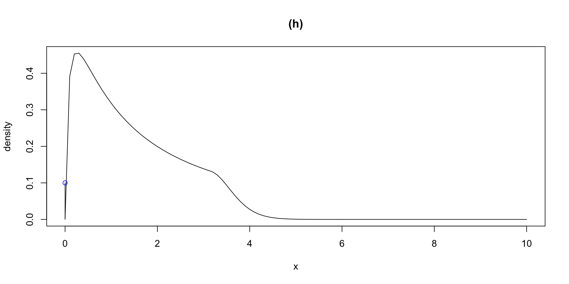
 dlogSST plogSST qlogSST rlogSST logSST

gen.Zadj(family="logSST")

A zero adjusted logSST distribution has been generated 
 and saved under the names:  
 dlogSSTZadj plogSSTZadj qlogSSTZadj rlogSSTZadj 
 plotlogSSTZadj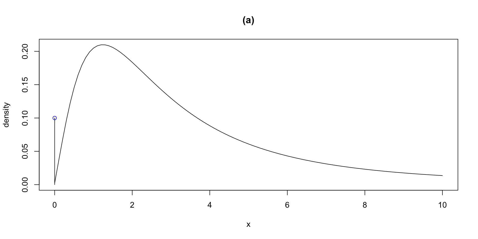

example zero adjusted (con.)

plotlogSSTZadj(mu= 1, sigma=1, nu=1, tau=10, xi0=.1); title("(a)")

example zero adjusted (con.)

plotlogSSTZadj(mu=-1, sigma=1, nu=1, tau=10, xi0=.1); title("(b)")

example zero adjusted (con.)

plotlogSSTZadj(mu=-1, sigma=2, nu=1, tau=10, xi0=.1); title("(c)")

example zero adjusted (con.)

plotlogSSTZadj(mu=0,  sigma=2, nu=1, tau=10, xi0=.1); title("(d)")

example zero adjusted (con.)

plotlogSSTZadj(mu=0,  sigma=1, nu=10,tau=10, xi0=.1); title("(e)")

example zero adjusted (con.)

plotlogSSTZadj(mu=0,  sigma=1, nu=1, tau=3,  xi0=.1); title("(f)")

example zero adjusted (con.)

plotlogSSTZadj(mu=0,  sigma=1, nu=2, tau=3,  xi0=.5); title("(g)")

example zero adjusted (con.)

plotlogSSTZadj(mu=0,  sigma=1, nu=.3,tau=100,xi0=.1); title("(h)")

Zero and one inflated distributions

\[\begin{eqnarray} f_Y(y)=\left\{ \begin{array}{ll} p_0 & \mbox{if $y=0$} \\ (1-p_0-p_1) f_W(y) & \mbox{if $0<y<1$} \\ p_1 & \mbox{if $y=1$} \\ \end{array} \label{pdfDINF} \right. \end{eqnarray}\]

example of Zero and one inflated

library(gamlss.dist)
plotBEINF( mu =.5 , sigma=.5, nu = 0.5, tau = 0.5)

example of Zero and one inflated (con.)

library(gamlss.inf)
gen.Family(family="SST", type="logit")

A  logit  family of distributions from SST has been generated 
 and saved under the names:  
 dlogitSST plogitSST qlogitSST rlogitSST logitSST

gen.Inf0to1(family="logitSST",  type.of.Inflation="Zero&One")

A  0to1 inflated logitSST distribution has been generated 
 and saved under the names:  
 dlogitSSTInf0to1 plogitSSTInf0to1 qlogitSSTInf0to1 rlogitSSTInf0to1 
 plotlogitSSTInf0to1

example of Zero and one inflated (con.)

plotlogitSSTInf0to1(mu= 1, sigma=1, nu=1, tau=10, xi0=.1, xi1=.2); title("(a)")

example of Zero and one inflated (con.)

plotlogitSSTInf0to1(mu=-1, sigma=1, nu=1, tau=10, xi0=.1, xi1=.2); title("(b)")

example of Zero and one inflated (con.)

plotlogitSSTInf0to1(mu=-1, sigma=2, nu=1, tau=10, xi0=.1, xi1=.2); title("(c)")

example of Zero and one inflated (con.)

plotlogitSSTInf0to1(mu=0,  sigma=2, nu=1, tau=10, xi0=.1, xi1=.2); title("(d)")

example of Zero and one inflated (con.)

plotlogitSSTInf0to1(mu=0,  sigma=1, nu=10,tau=10, xi0=.1, xi1=.2); title("(e)")

example of Zero and one inflated (con.)

plotlogitSSTInf0to1(mu=0,  sigma=1, nu=1, tau=3,  xi0=.1, xi1=.2); title("(f)")

example of Zero and one inflated (con.)

plotlogitSSTInf0to1(mu=0,  sigma=1, nu=2, tau=3,  xi0=.5, xi1=.1); title("(g)")

example of Zero and one inflated (con.)

plotlogitSSTInf0to1(mu=0,  sigma=1, nu=.3,tau=100,xi0=.1, xi1=.5); title("(h)")

select distribution

Find a distribution

flowchart TB
  A[responce] --> B(continuous) 
  A --> C[discrete]
  A --> D[factor]
  B --> F[real line]
  B --> G[pos. real line]
  B --> H[0 to 1]
  C --> J[infinite count]
  C --> I[finite count]
  D --> K[unordered]
  D --> L[ordered]
  I --> N[binary]
  K --> N[binary]

Figure 1: Type of distribution for the response.

Summary

Select an appropriate class of distributions following the diagram above.
Use the function chooseDist() to fit a “linear” models for both $\mu$ and $\sigma$
Use GAIC to finds the best fit
Use model diagnostics to check the distribution

`chooseDist()`

library(gamlss2)
da <- rent99[, -c(2,9)]
# fit a linear model with all variables above to both mu and sigma
 m1 <- gamlss2(rent~.|., data=da, family=GA,trace=FALSE)
 M1 <- chooseDist(m1, type="realplus", parallel="snow", ncpus=10)

minimum GAIC(k= 2 ) family: BCTo 
minimum GAIC(k= 3.84 ) family: BCCGo 
minimum GAIC(k= 8.03 ) family: BCCGo

`chooseDist()` (con.)

getOrder(M1, column=1)

GAIG with k= 2

    BCTo    BCCGo    BCPEo       GG      GB2     BCCG      BCT     BCPE 
38435.06 38435.48 38436.67 38448.83 38469.66 38474.04 38475.64 38476.00 
      GA   exGAUS      WEI     WEI3      GIG    LOGNO   LOGNO2       IG 
38485.04 38513.62 38517.73 38518.44 38548.69 38633.88 38633.88 38695.74 
    WEI2      EXP  PARETO2       GP PARETO2o   IGAMMA      LNO 
38905.86 43706.40 44005.87 44005.87 46106.69 66406.55       NA

worm plot

Figure 2

bucket plot

Summary

flowchart LR
  A(responce) --> B[type] 
  B --> C[initial fit]
  C --> D[chooseDist]
  D --> F{check}
  F --> G[residual diagnostics]
  F --> E[overfitting]

Figure 3: Summary for finding an initial distribution.

practical 3

END

back to the index

The Books

name	gamlss	range	parameter-links
beta inf.	`BEINF0`	\([0, 1)\)	logit , logit , log , -
beta-inf.	`BEOI`	\([0 , 1)\)	logit , log , logit , -
beta 1-inf.	`BEINF1`	\((0, 1]\)	logit , logit , log , -
beta 1-inf.	`BEZI`	\((0, 1]\)	logit, log, logit, -
beta 0 & 1 inf	`BEINF`	\([0, 1]\)	logit, logit, log, log
gamma 0-adj.	`ZAGA`	\([0, \infty)\)	log, log, logit, -
inv Gaussian 0-adj	`ZAIG`	\([0, \infty)\)	log, log, logit, -

Mixed Distributions

introduction

Types

Zero adjusted distributions

Zero adjusted distributions

Explicit mixed dist (con.)

zero adjusted

zero adjusted con.

example zero adjusted

example zero adjusted (con.)

example zero adjusted (con.)

example zero adjusted (con.)

example zero adjusted (con.)

example zero adjusted (con.)

example zero adjusted (con.)

example zero adjusted (con.)

example zero adjusted (con.)

Zero and one inflated distributions

Zero and one inflated distributions

example of Zero and one inflated

example of Zero and one inflated (con.)

example of Zero and one inflated (con.)

example of Zero and one inflated (con.)

example of Zero and one inflated (con.)

example of Zero and one inflated (con.)

example of Zero and one inflated (con.)

example of Zero and one inflated (con.)

example of Zero and one inflated (con.)

example of Zero and one inflated (con.)

select distribution

Find a distribution

Summary

chooseDist()

chooseDist() (con.)

worm plot

bucket plot

Summary

practical 3

END

`chooseDist()`

`chooseDist()` (con.)