flowchart TB
  A[Features.] --> B(Parameters)
  B --> D[Properties, \n Characteristics]
  D -->  C(Distribution)
  B --> C
Interpreting models
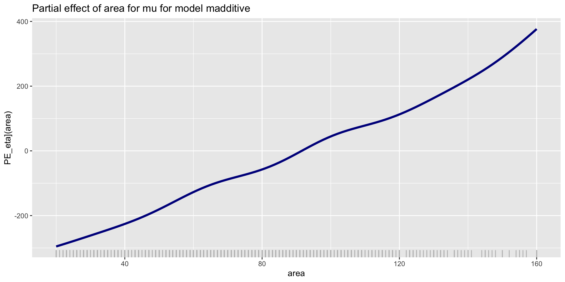
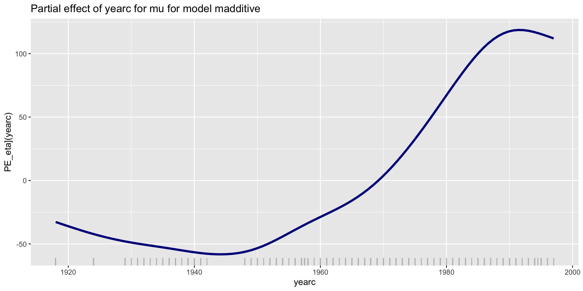
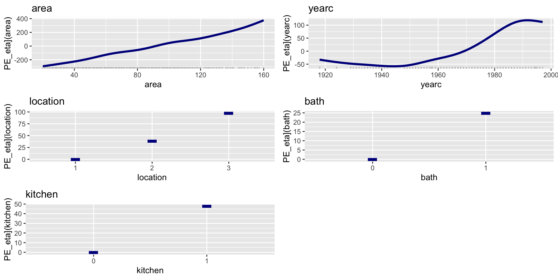
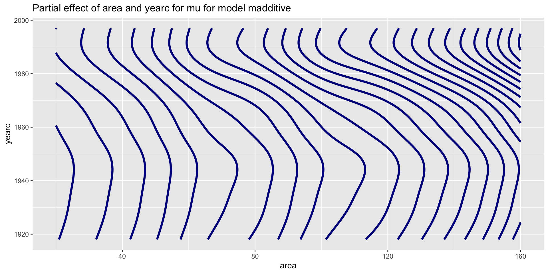
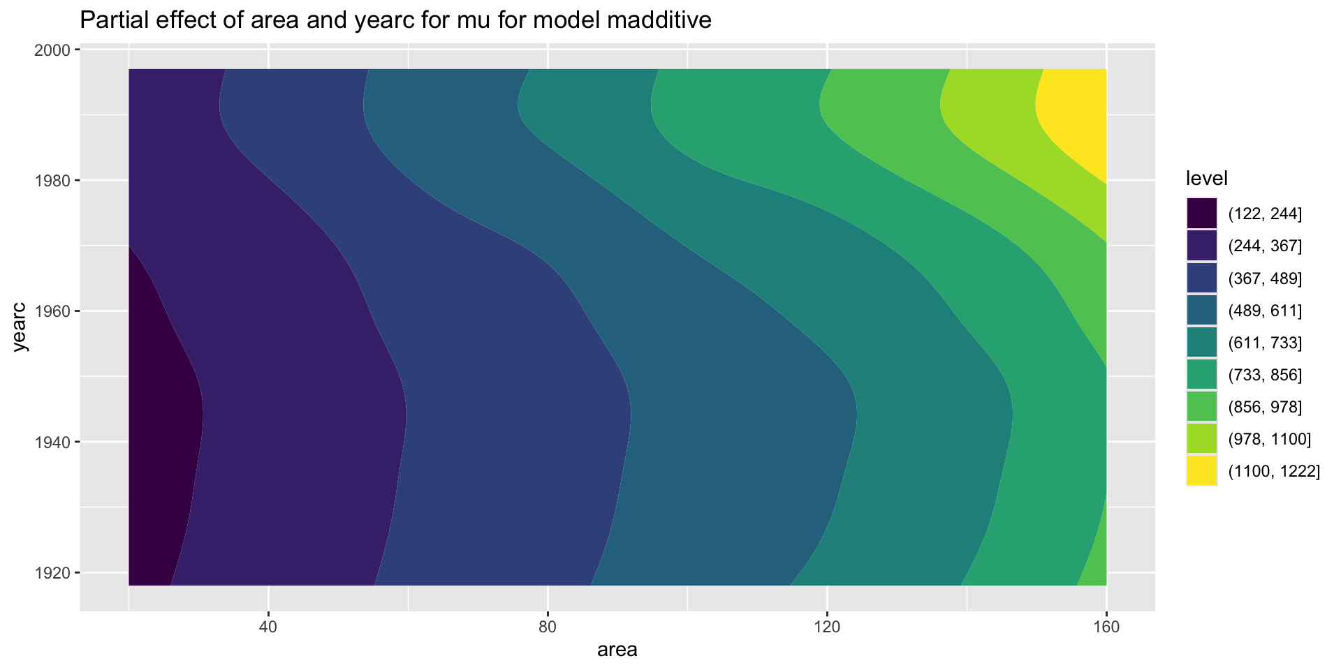
PE-parameter \(\mu\) additive
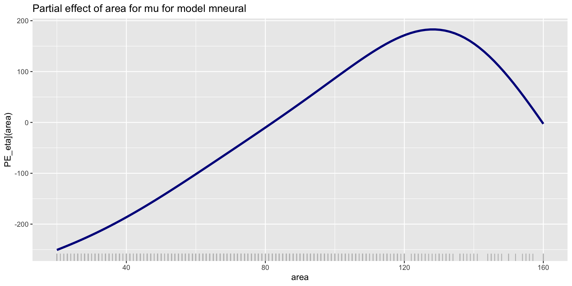
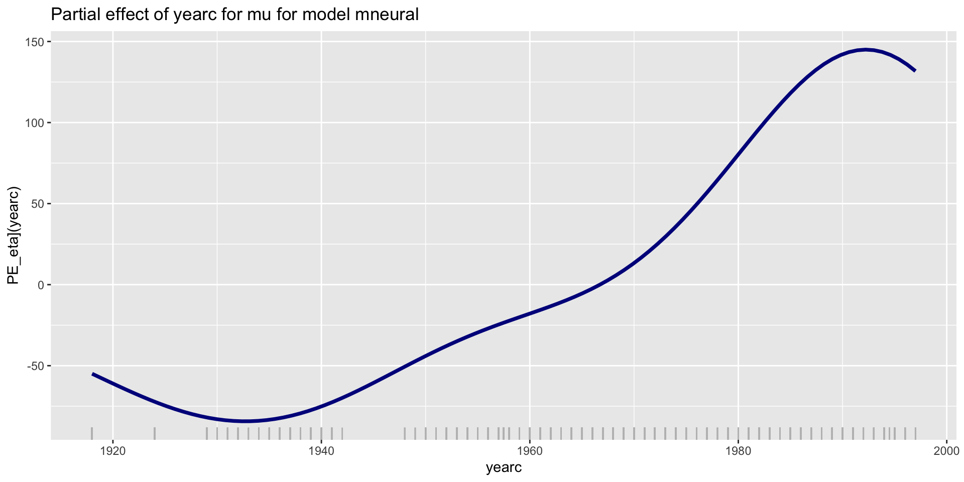
PE-parameter \(\mu\) NN
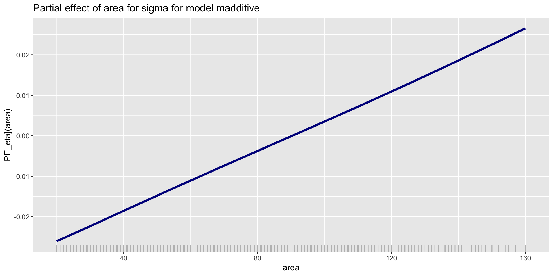
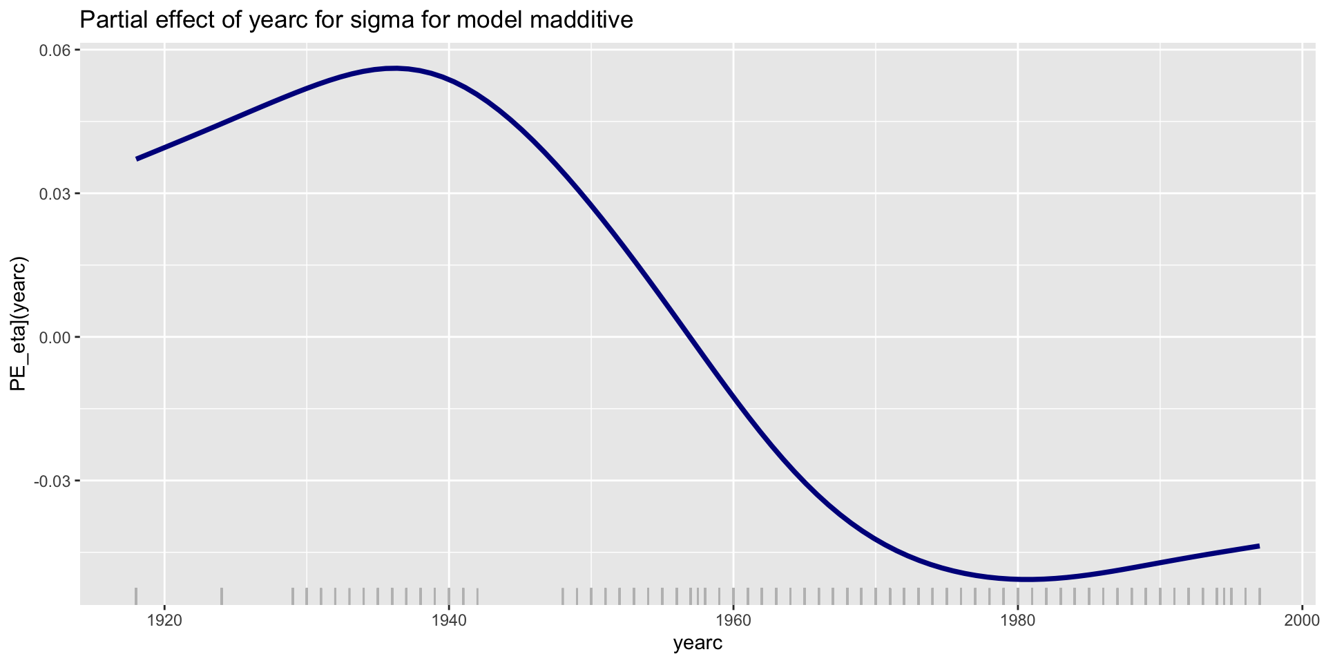
PE; parameter \(\sigma\); additive
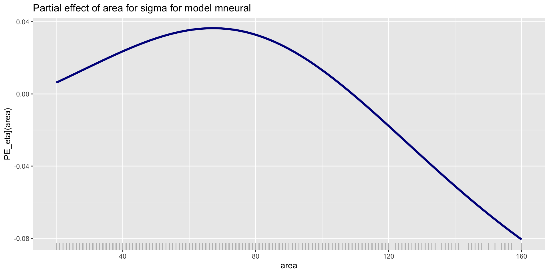
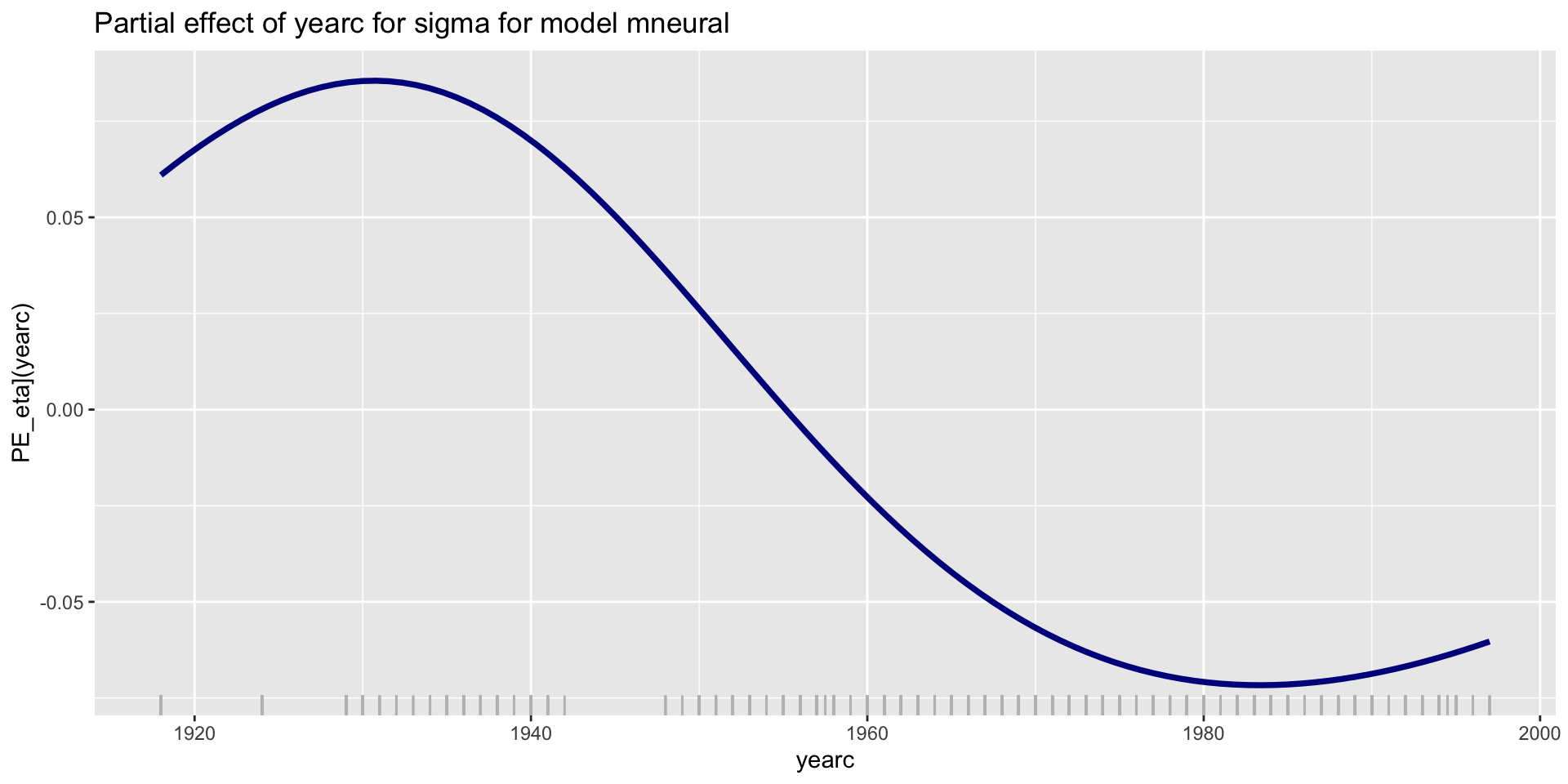
PE; parameter \(\sigma\); NN
all terms (additive)
2 way interactions (additive)
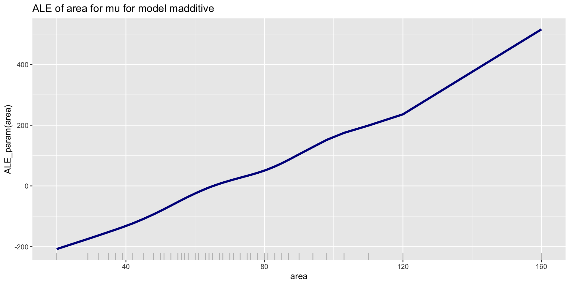
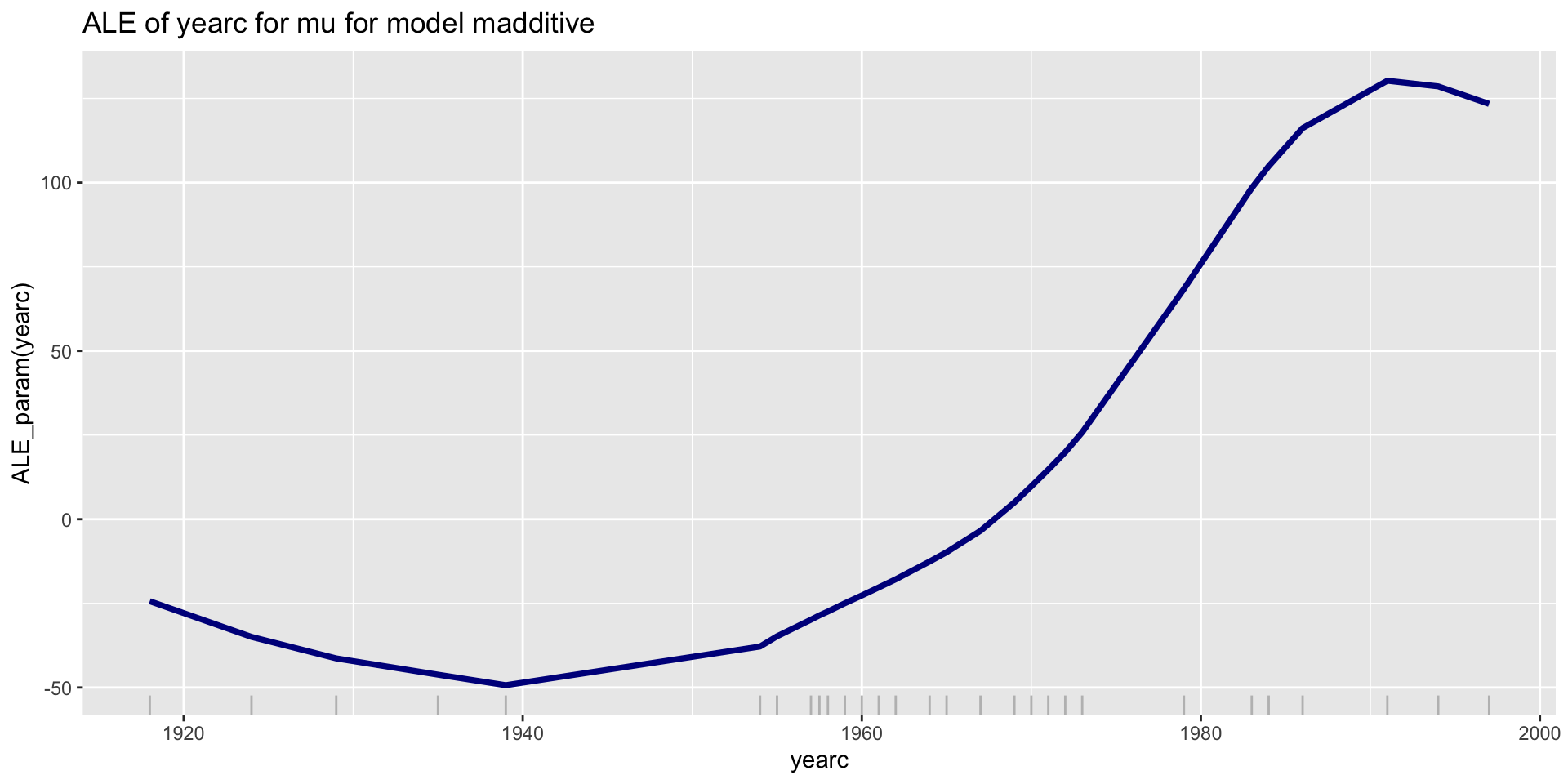
ALE; parameters \(\mu\); Additive
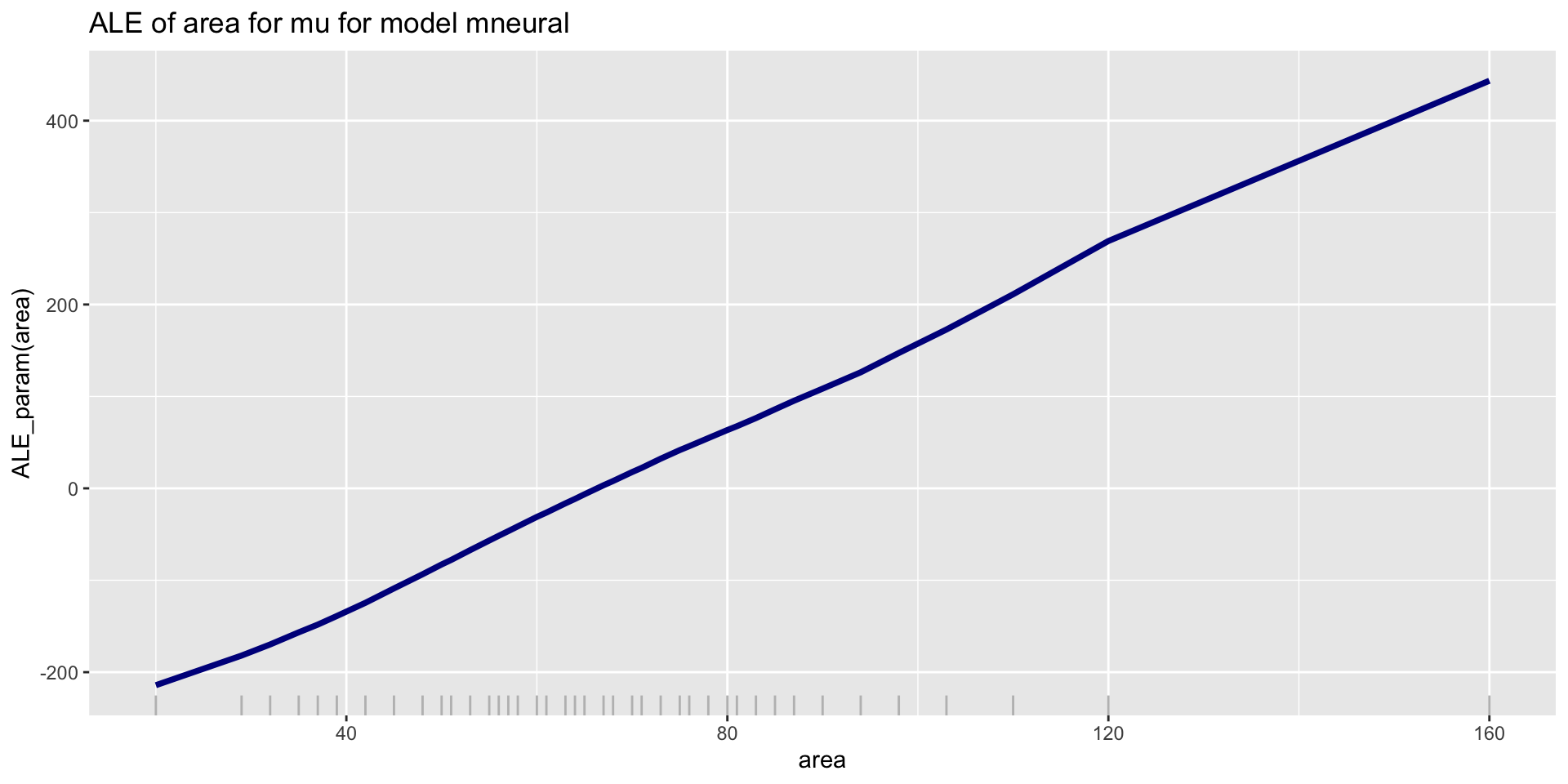
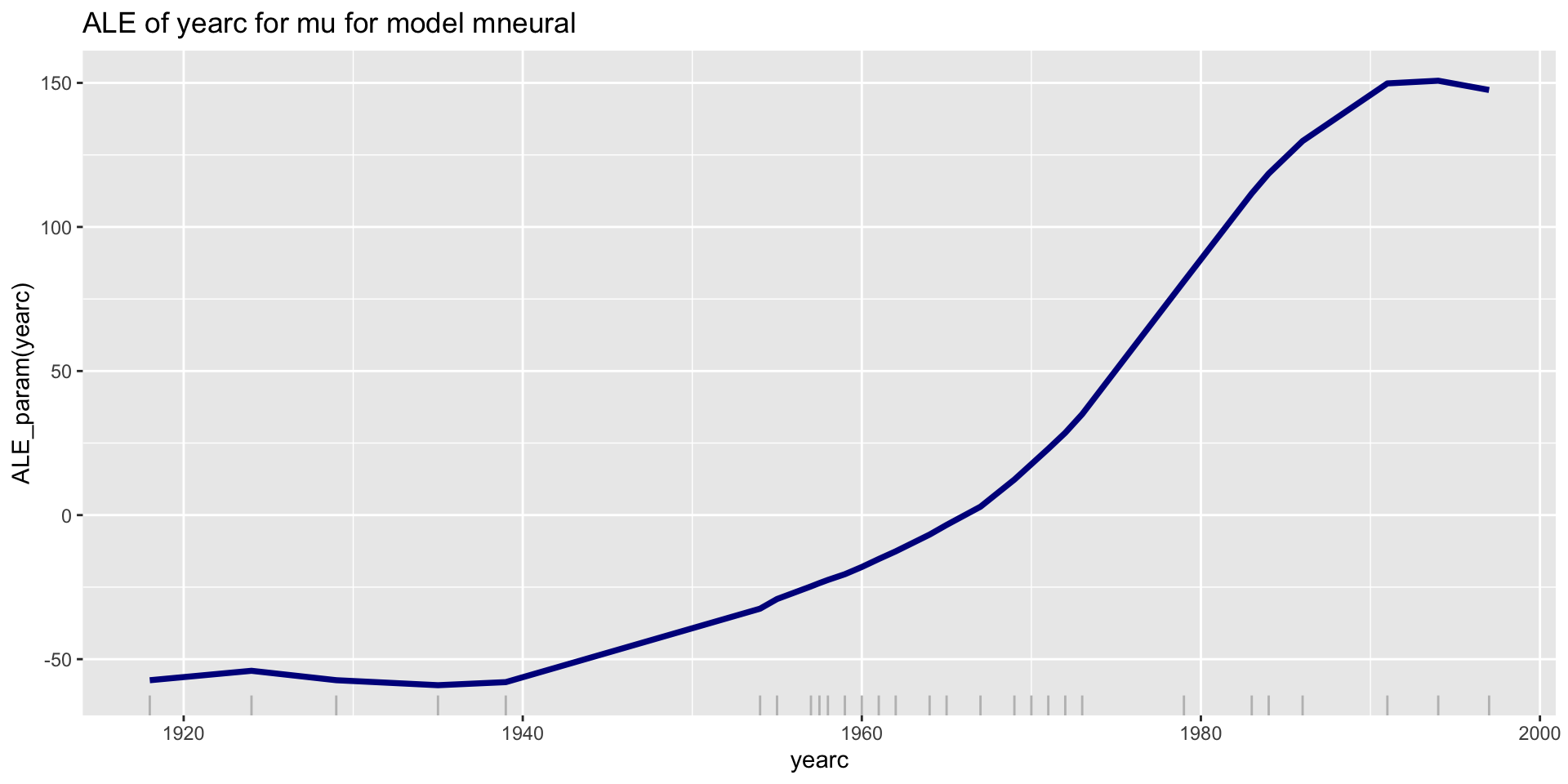
ALE; parameters \(\mu\); NN
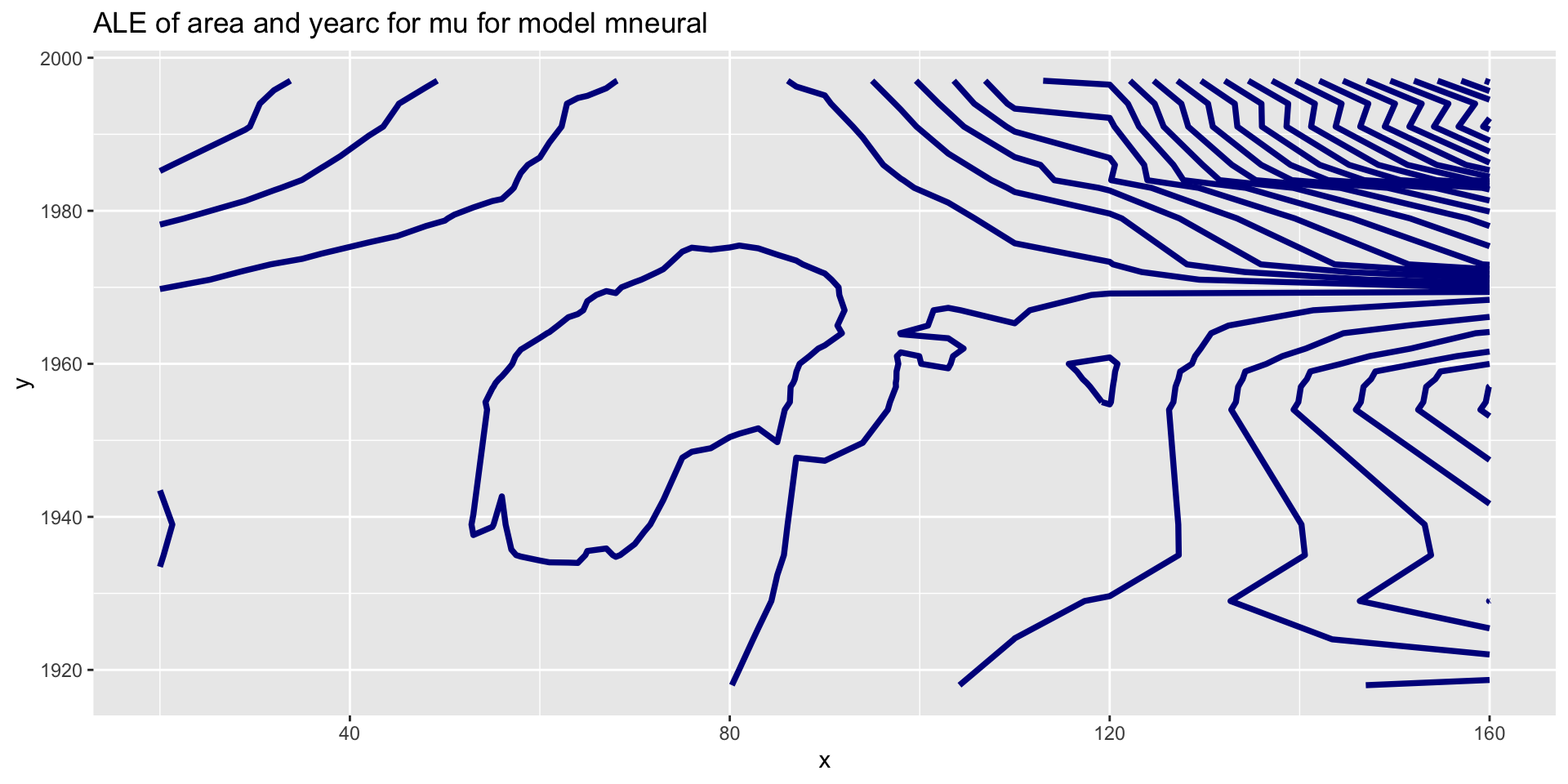
ALE interactions
gamlss.ggplots:::ale_param(madditive,c("area", "yearc"))
gamlss.ggplots:::ale_param(mneural,c("area", "yearc"))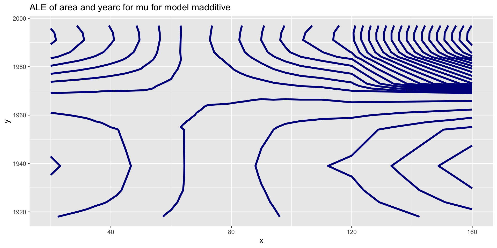
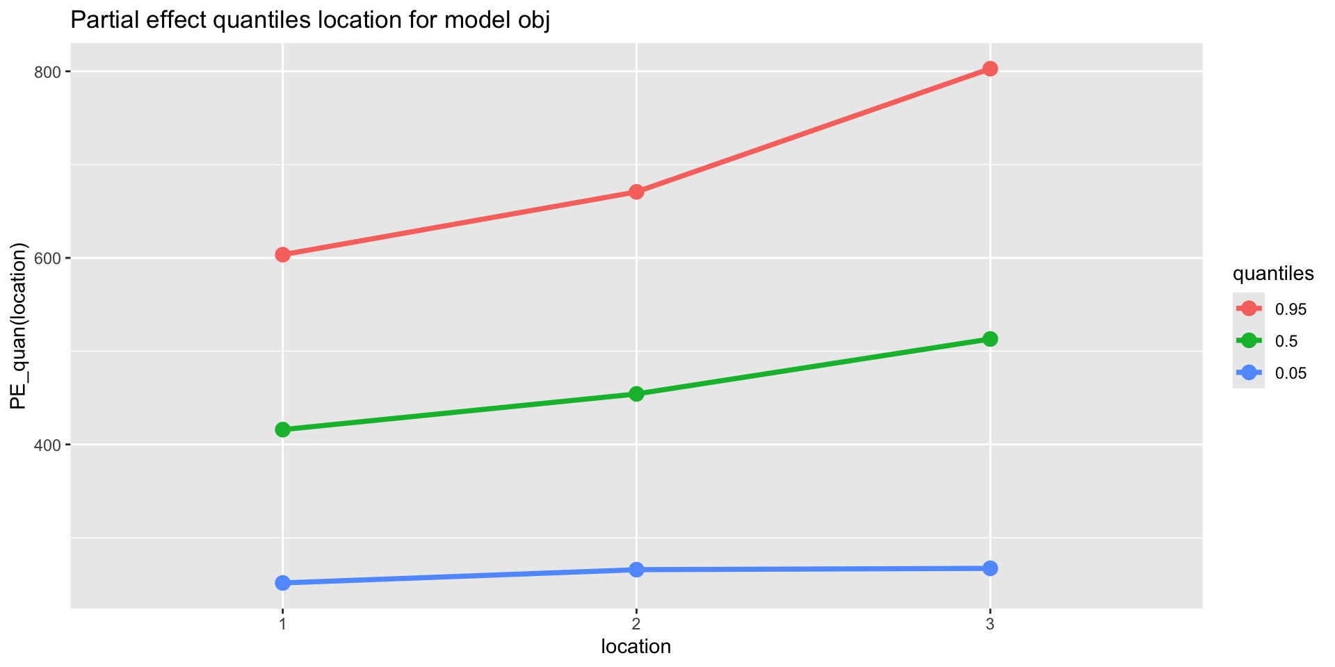
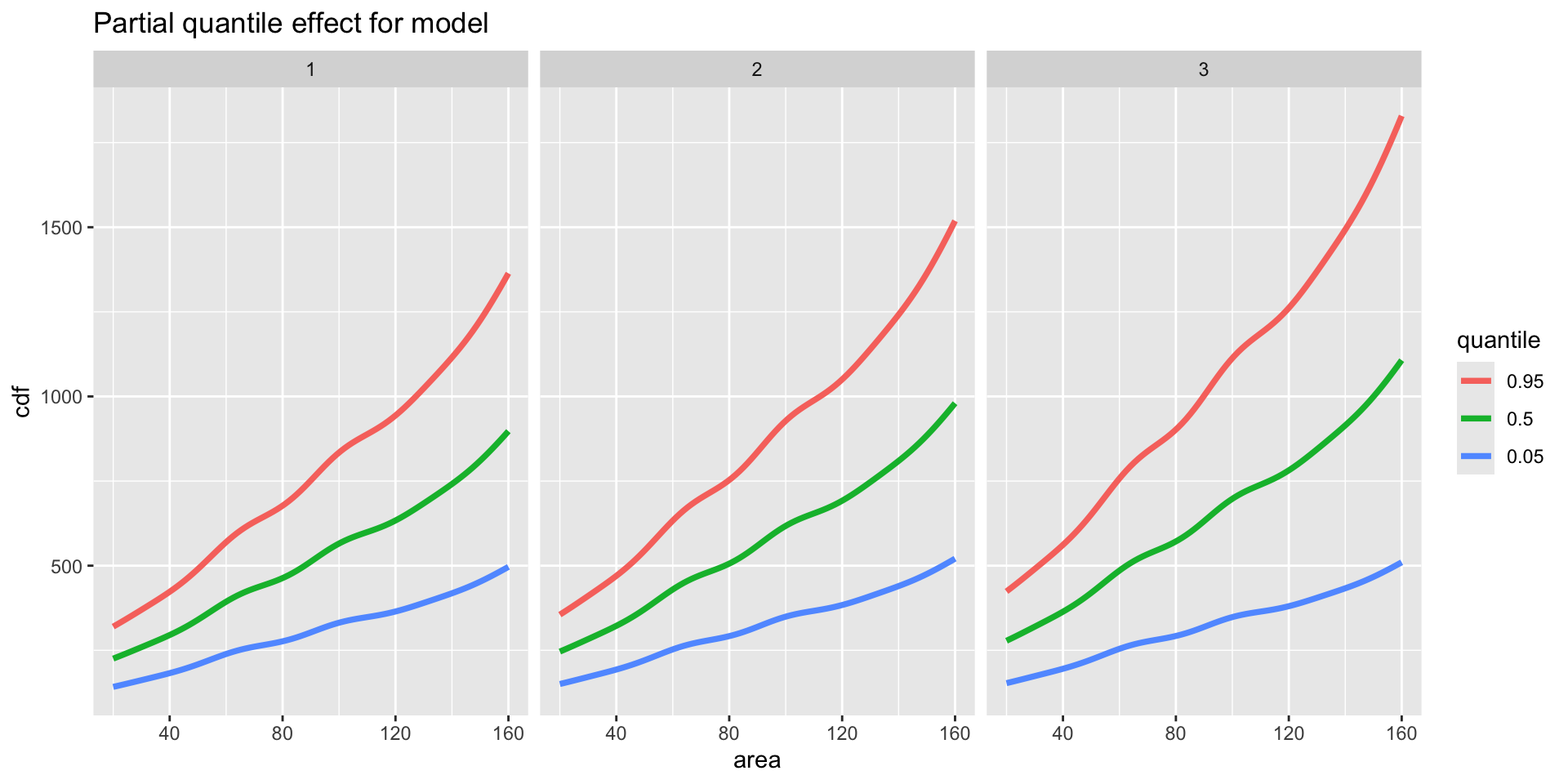
quantiles, additive
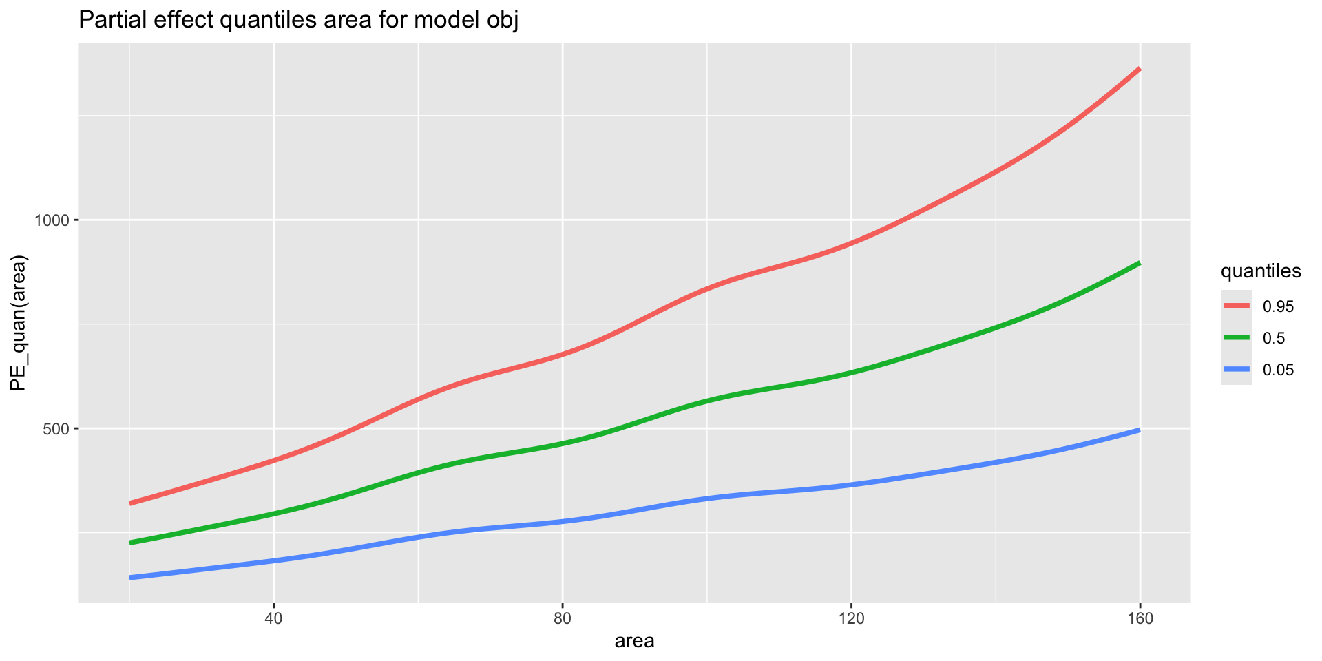
quantiles, additive (con.)
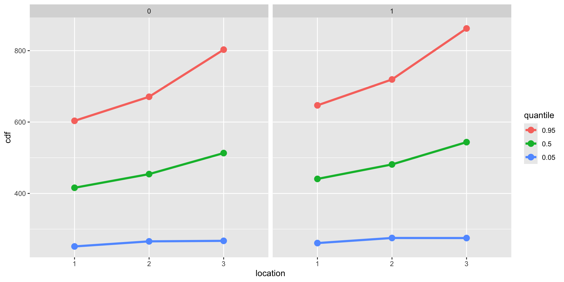
quantiles interactions
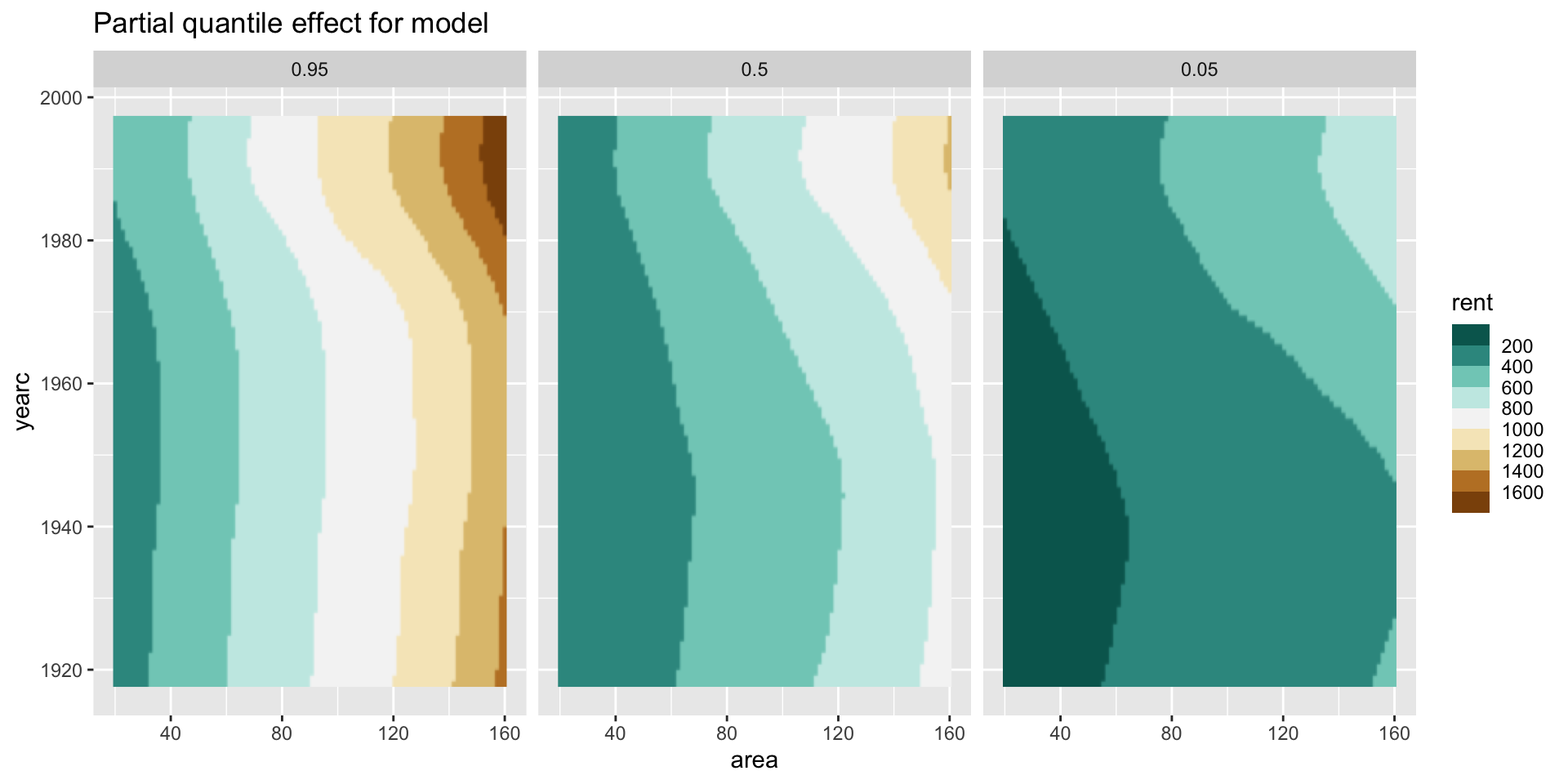
quantiles interactions 2
quantiles interactions 2
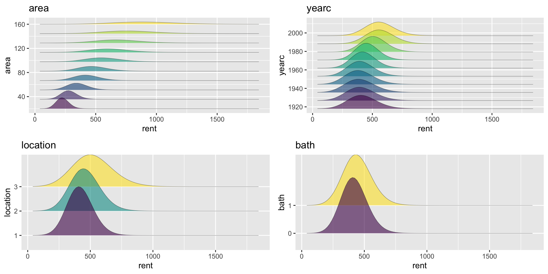
distributions, \(\mu\), additive
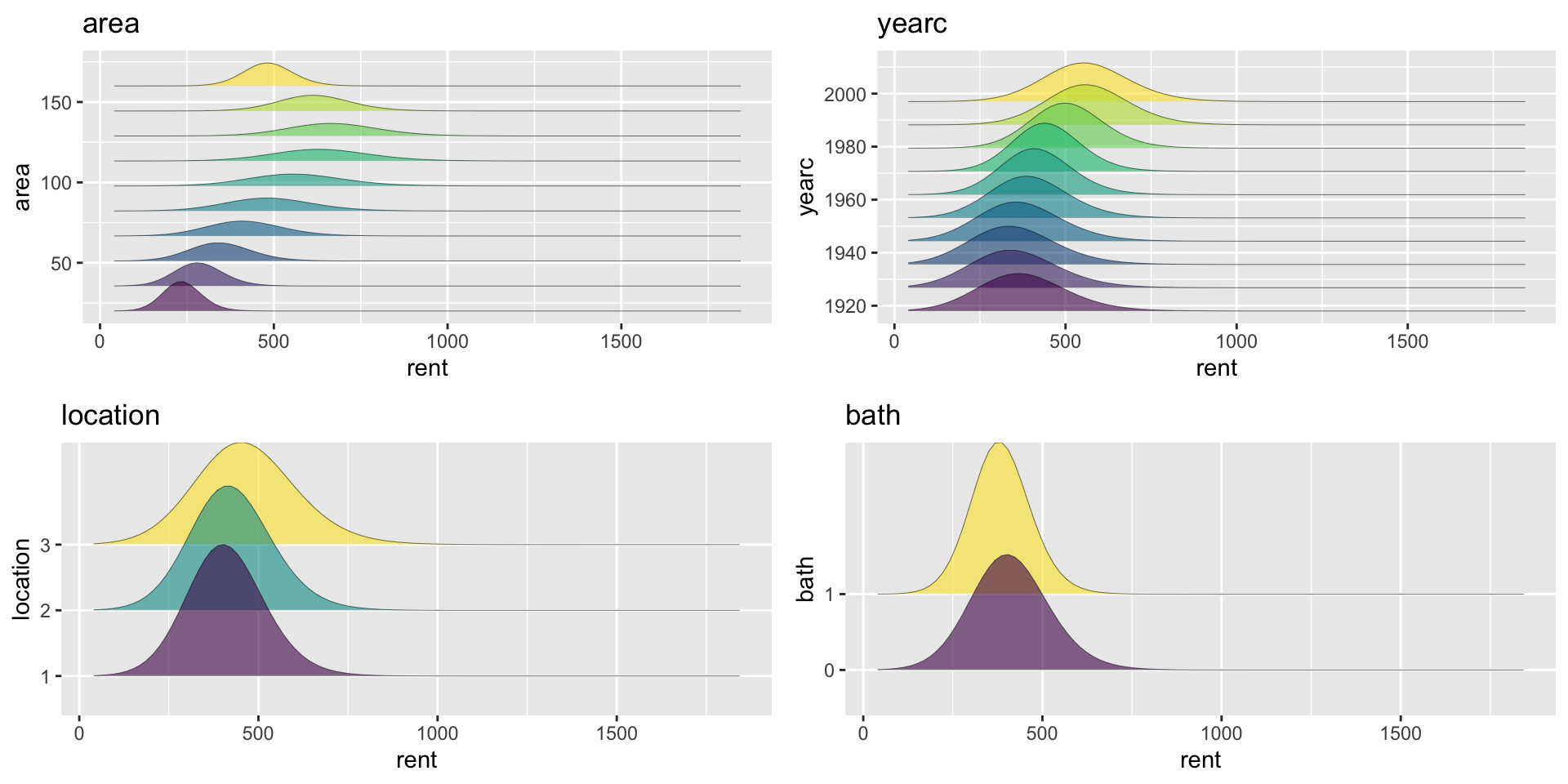
distributions, \(\mu\), NN
end
 The Books
![]()