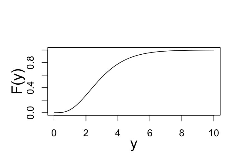
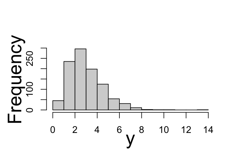
Distributions
continuous
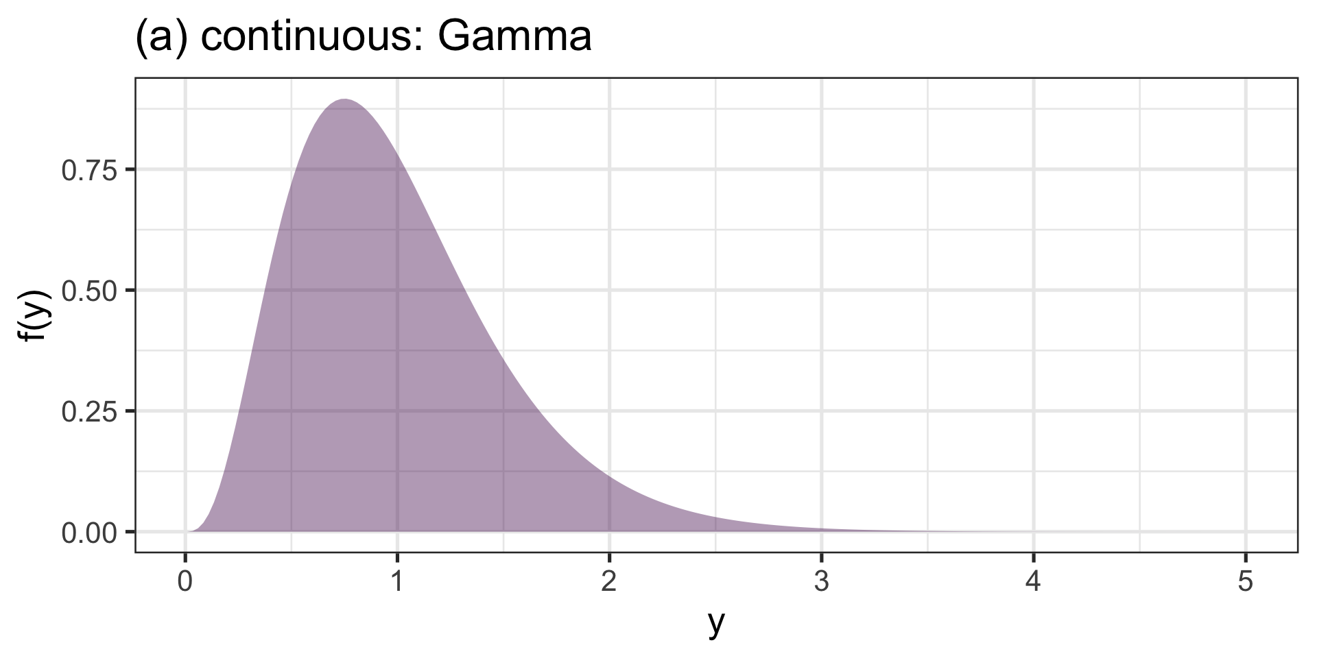
(a) continuous
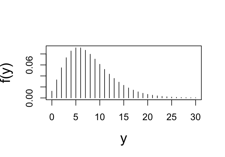
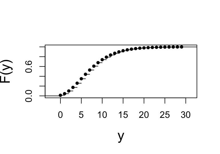
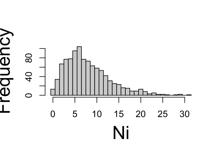
discrete
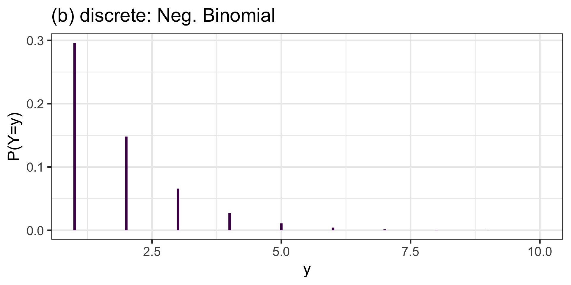
(a) discrete
mixed
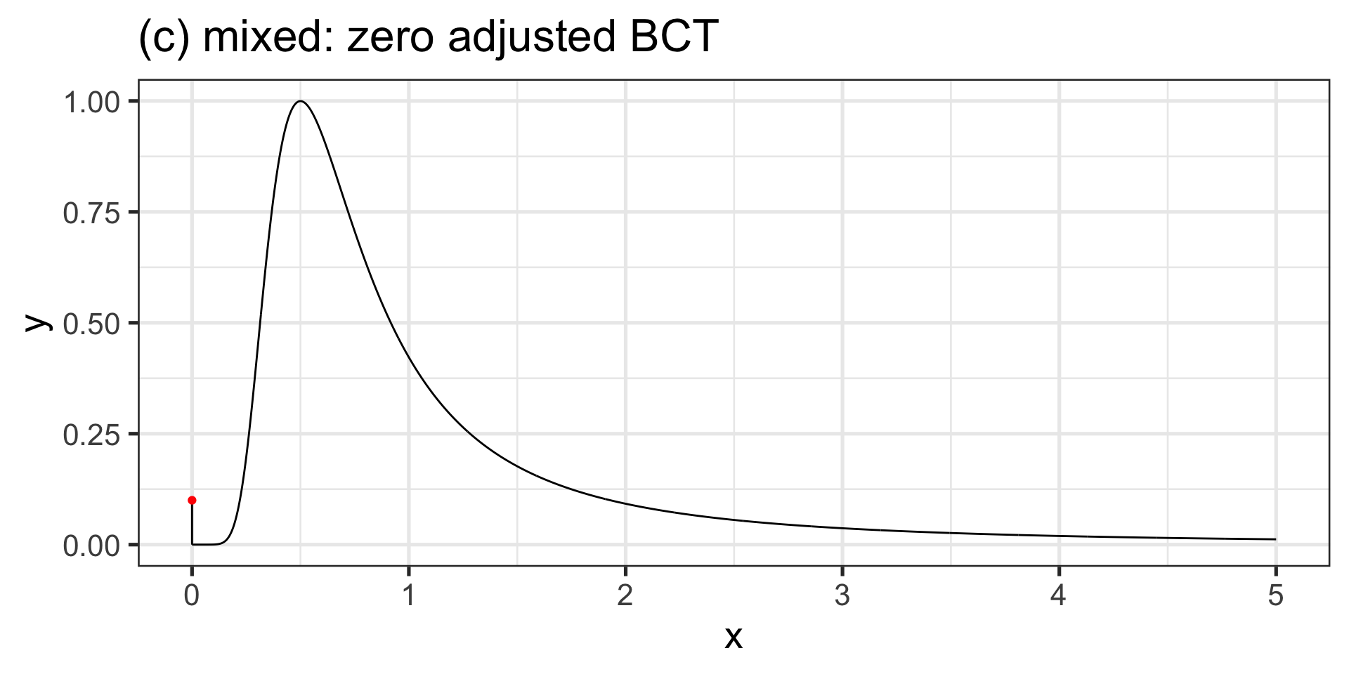
(a) mixed
left skew
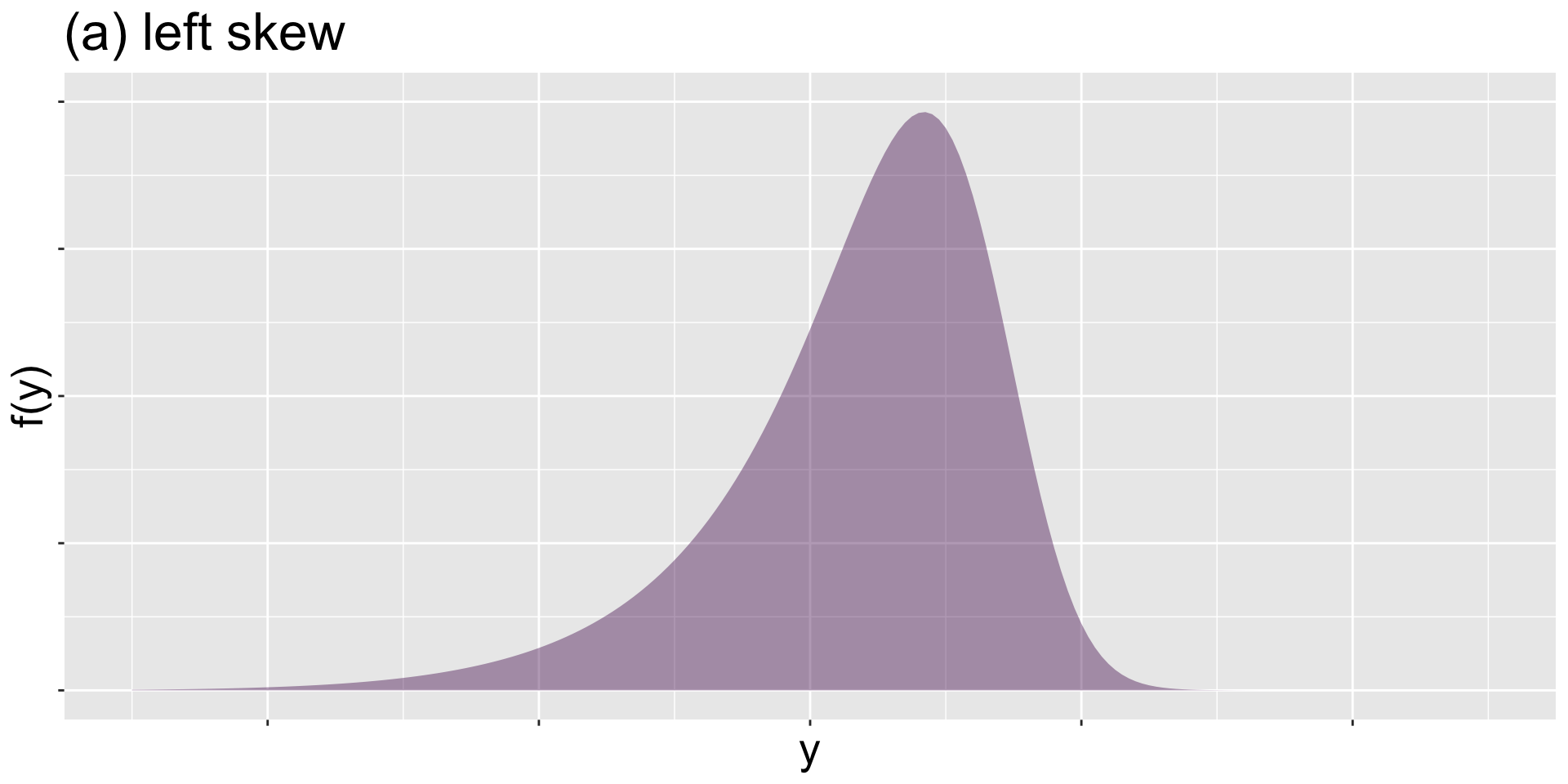
(a) left skew
symmetric
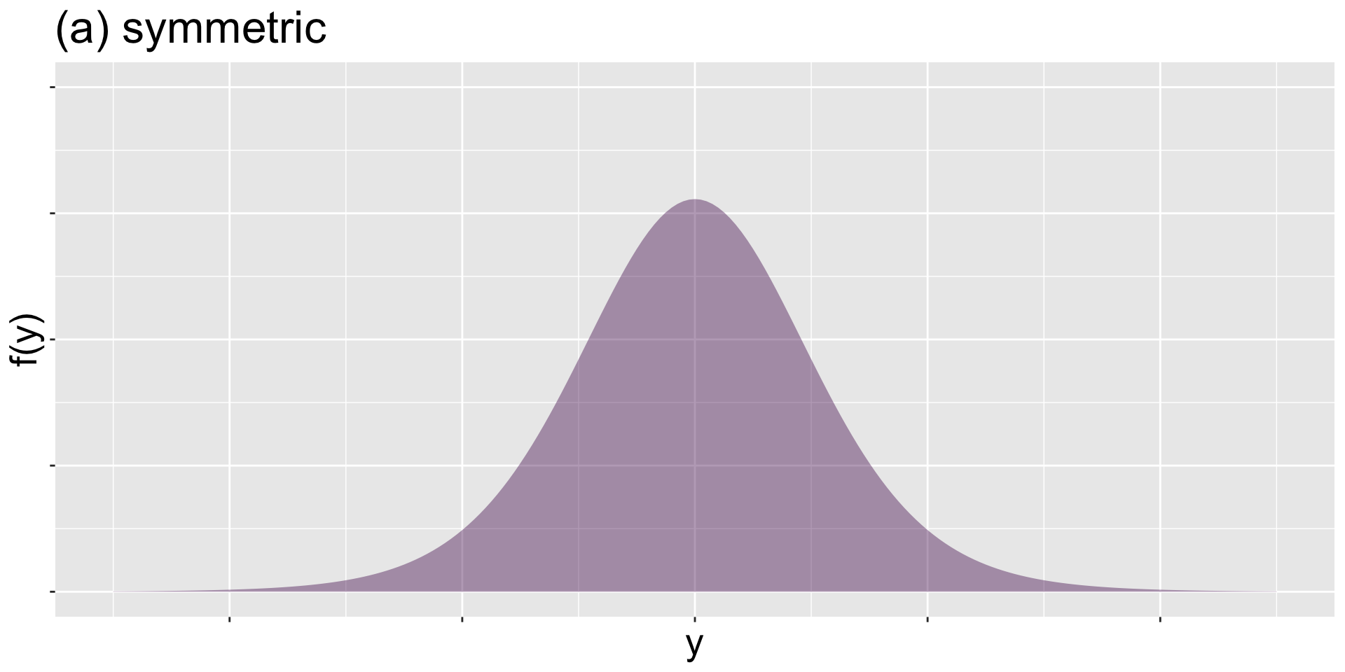
(a) symmetric
right skew
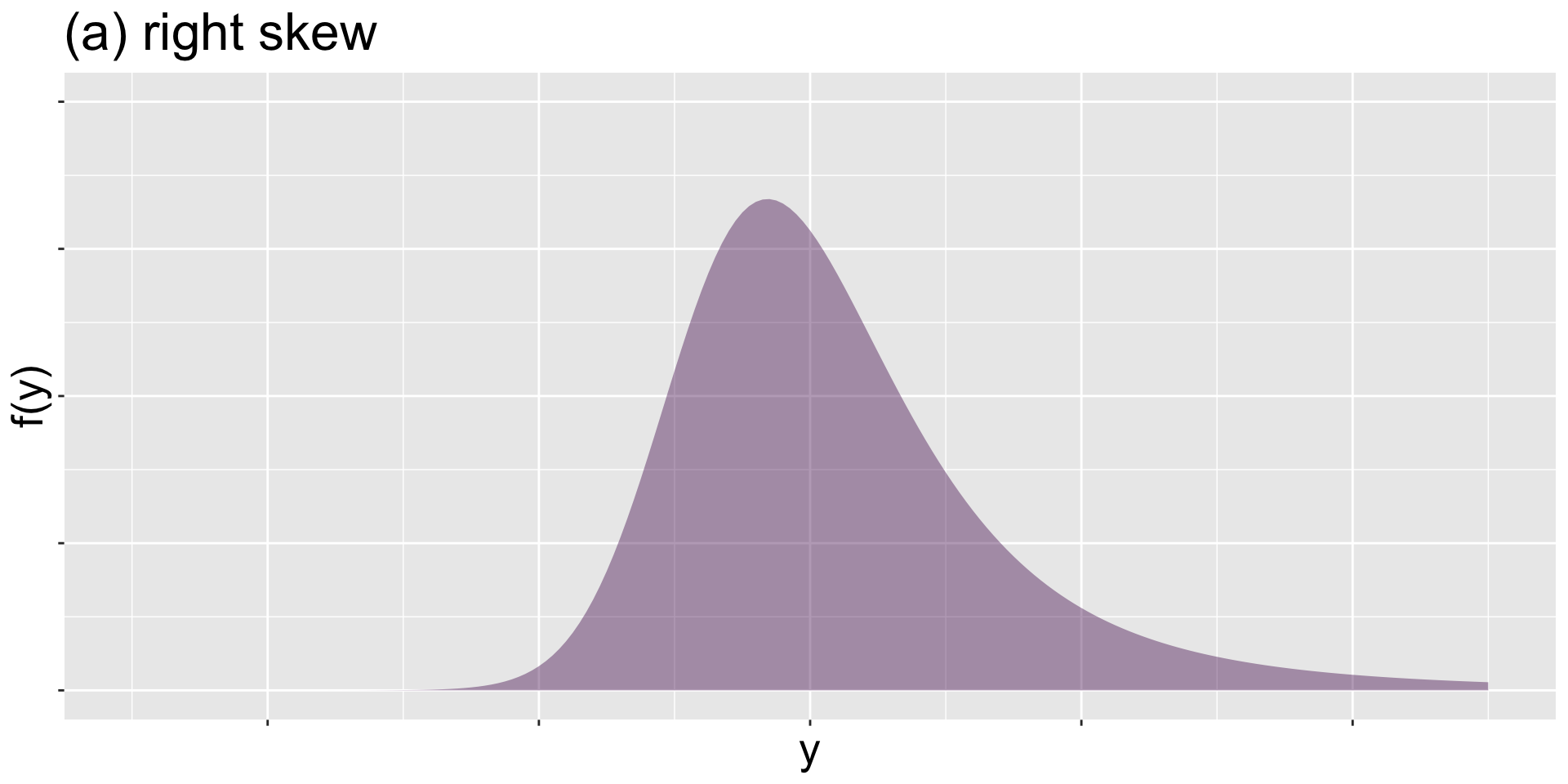
Figure 6: right skew
platy
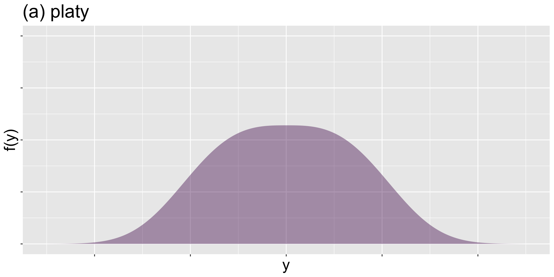
(a) platy
meso
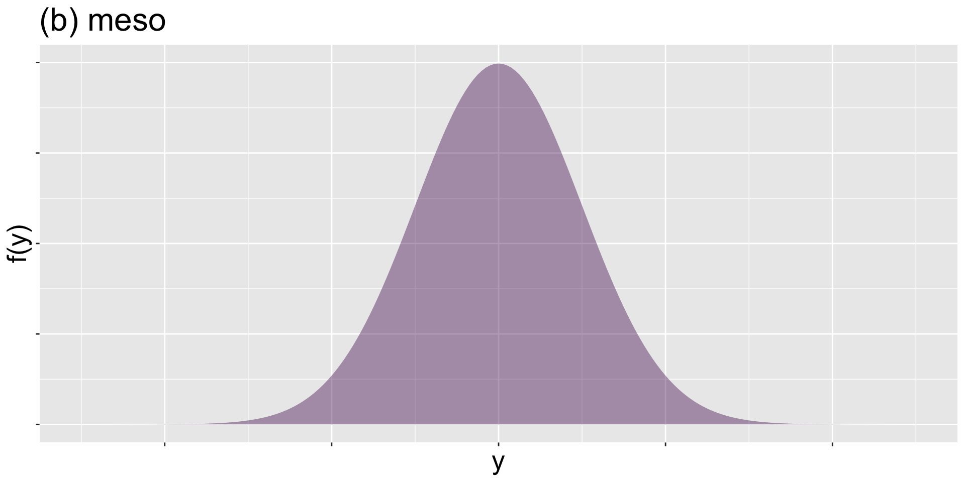
Figure 8: meso
lepto
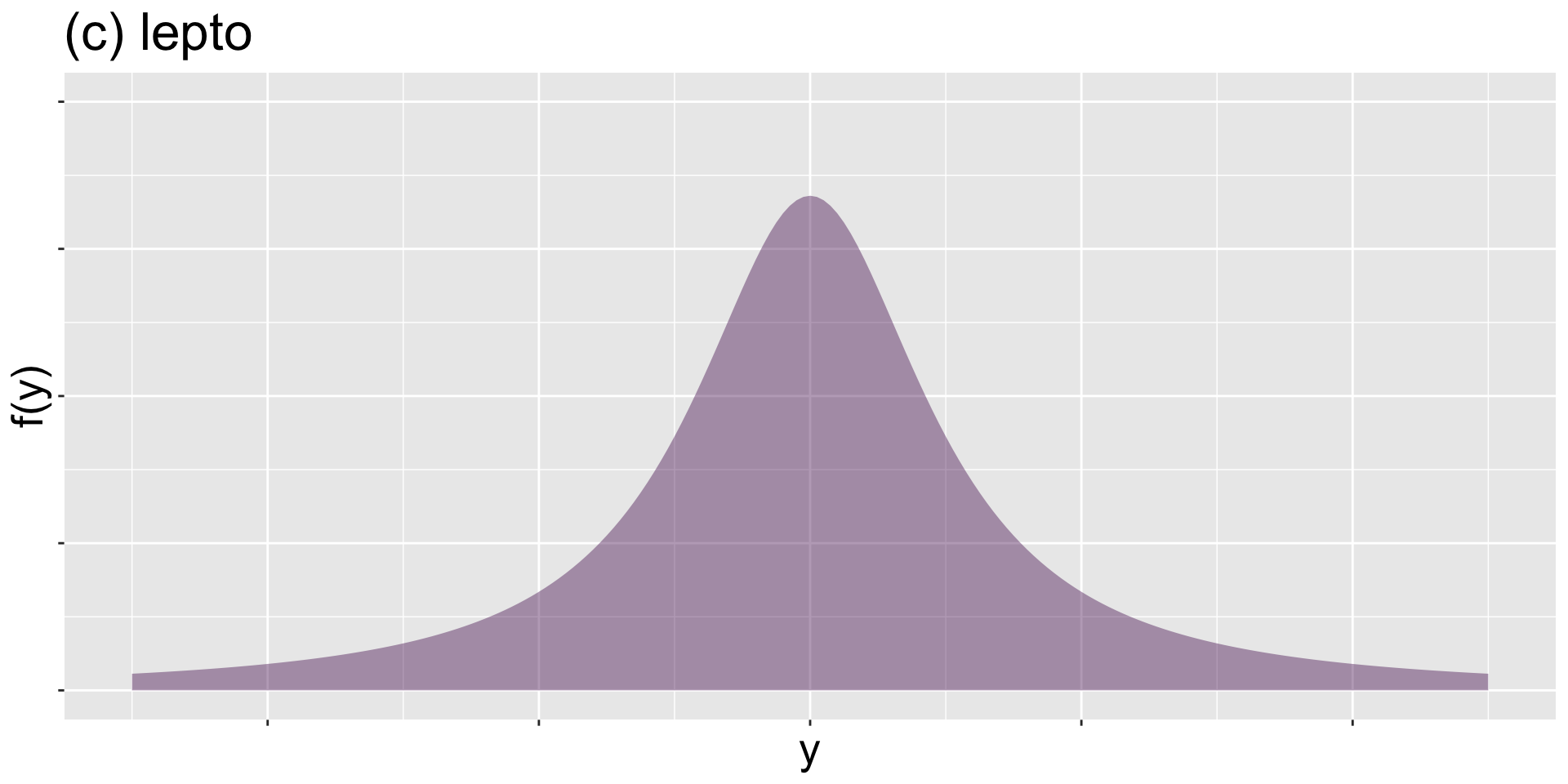
Figure 9: lepto
mean
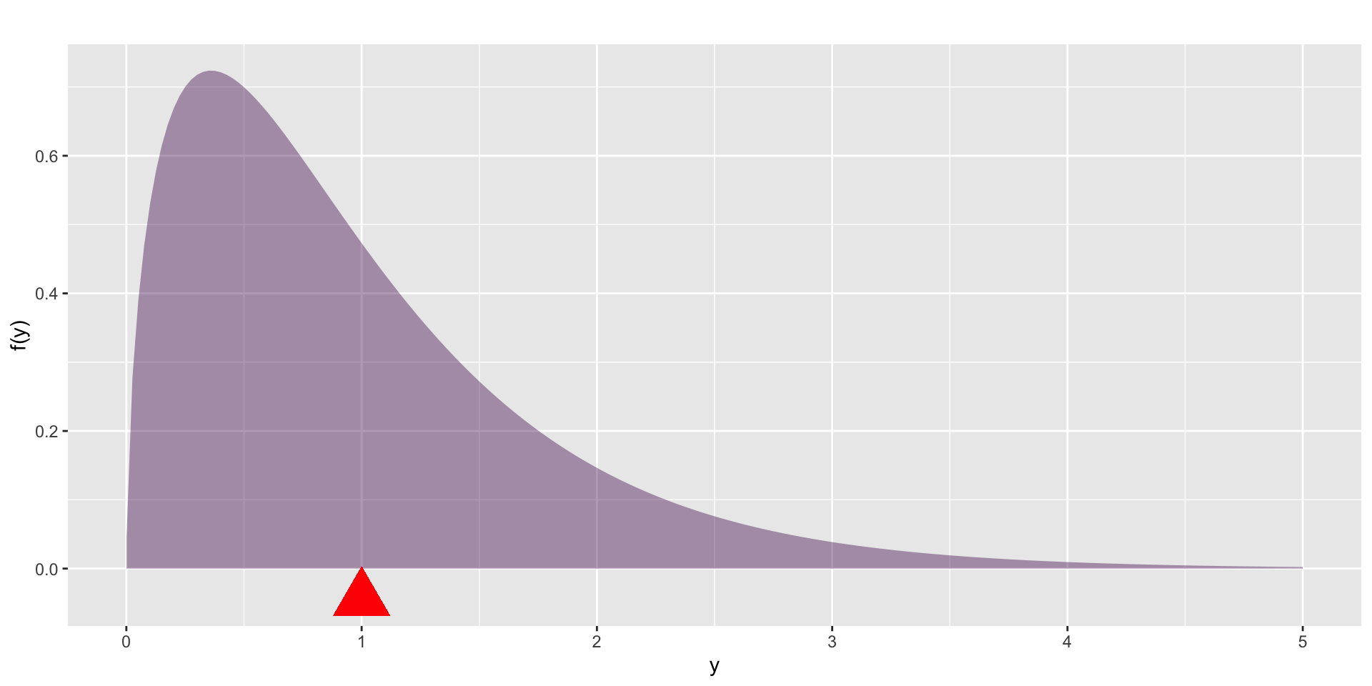
Figure 10: The mean is the point in which the distribution is balance.
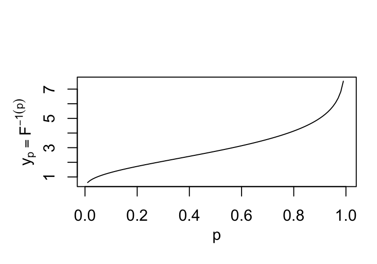
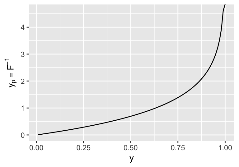
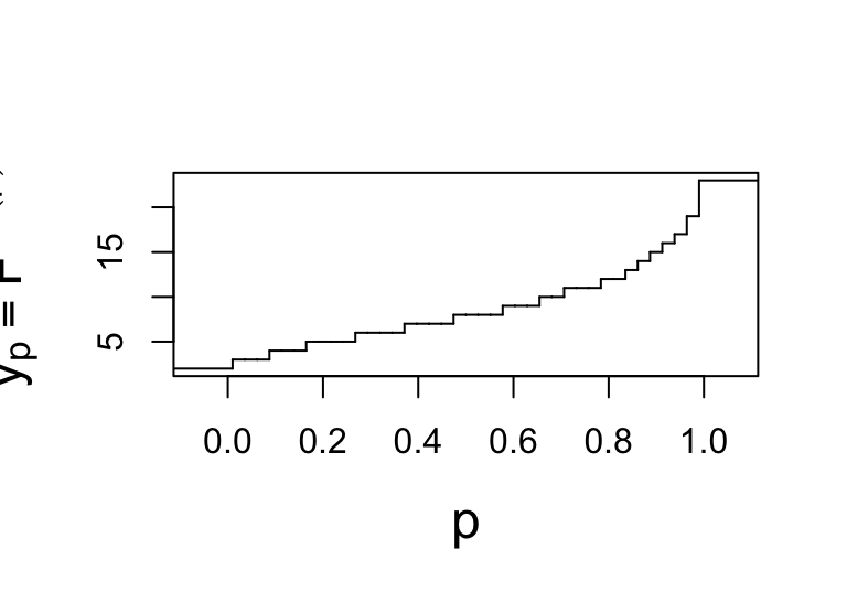
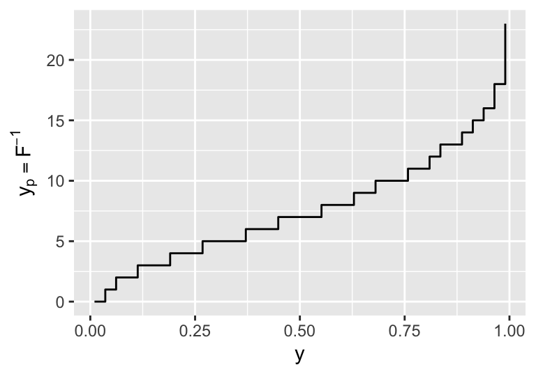
quantiles
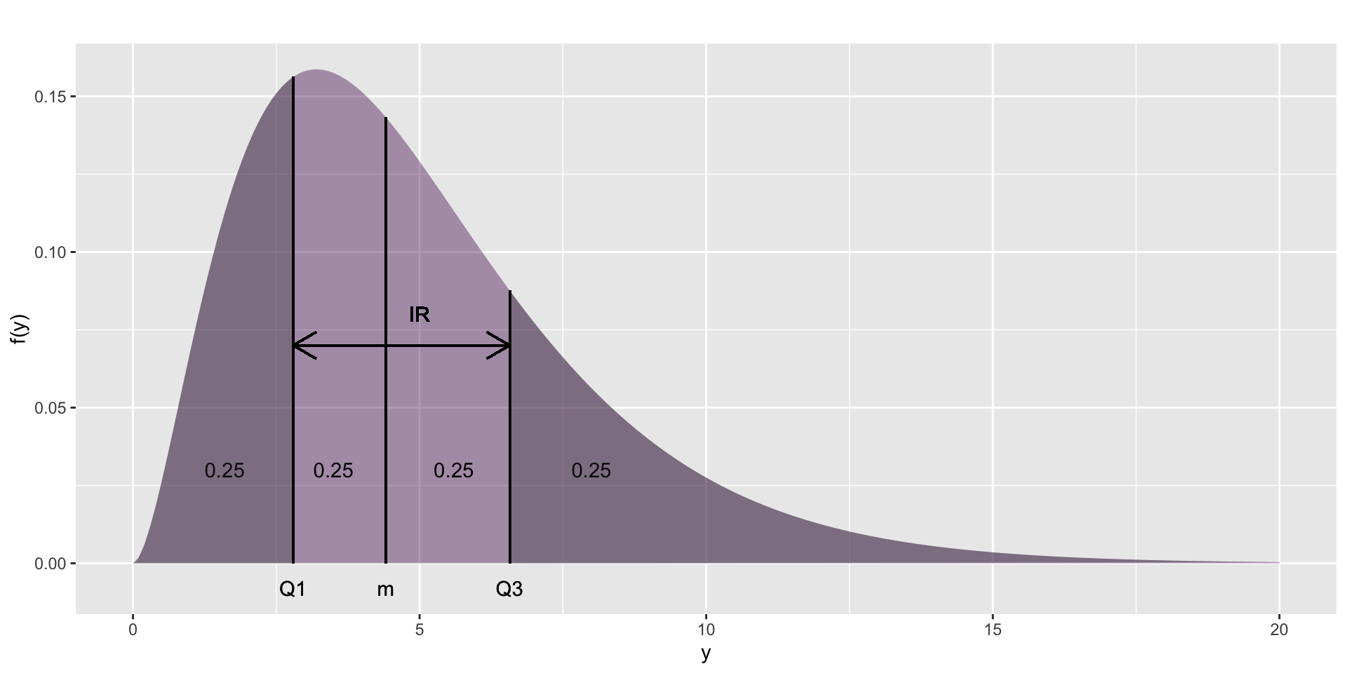
Figure 11: Showing how \(Q1\), \(m\) (median), \(Q3\) and the interquartile range IR of a continuous distribution are derived from \(f(y)\).
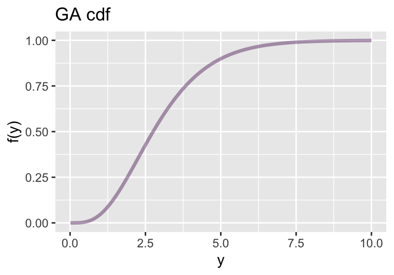
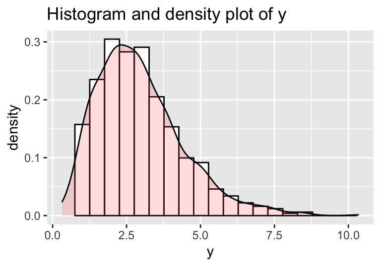
continuous
with ggplot2

discrete
with ggplot2
truncated continuous
A truncated family of distributions from NO has been generated
 and saved under the names:
 dNOtr pNOtr qNOtr rNOtr NOtr
The type of truncation is both
and the truncation parameter is 0 3 1 with absolute error < 1.1e-14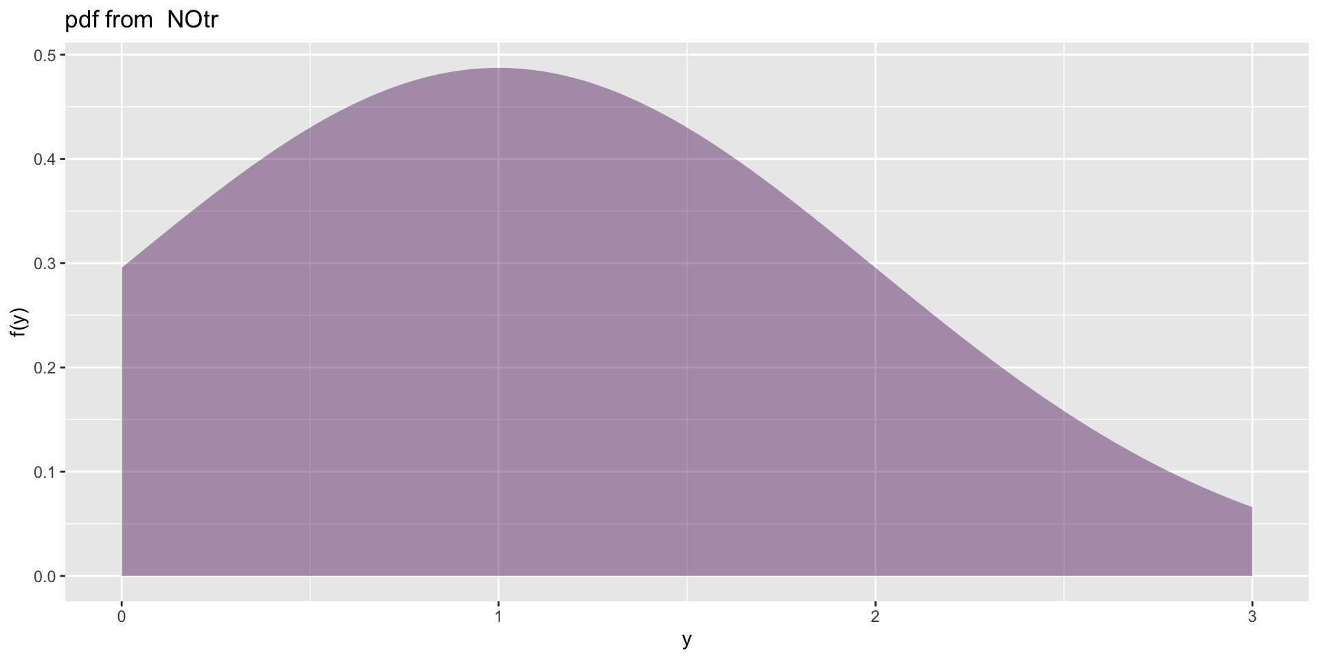
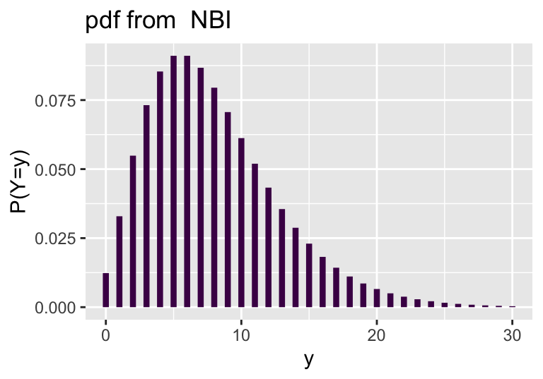
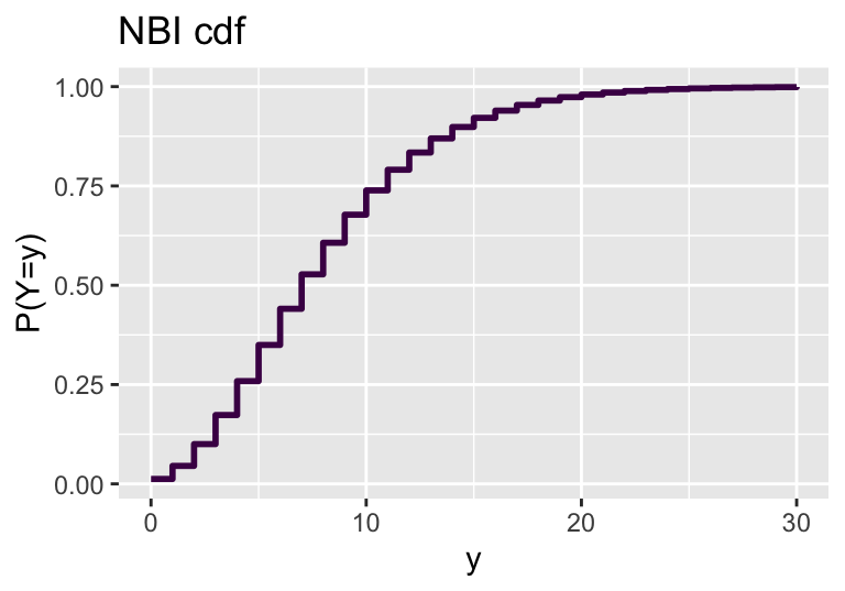
truncated discrete
A truncated family of distributions from NBI has been generated
 and saved under the names:
 dNBItr pNBItr qNBItr rNBItr NBItr
The type of truncation is left
and the truncation parameter is 0 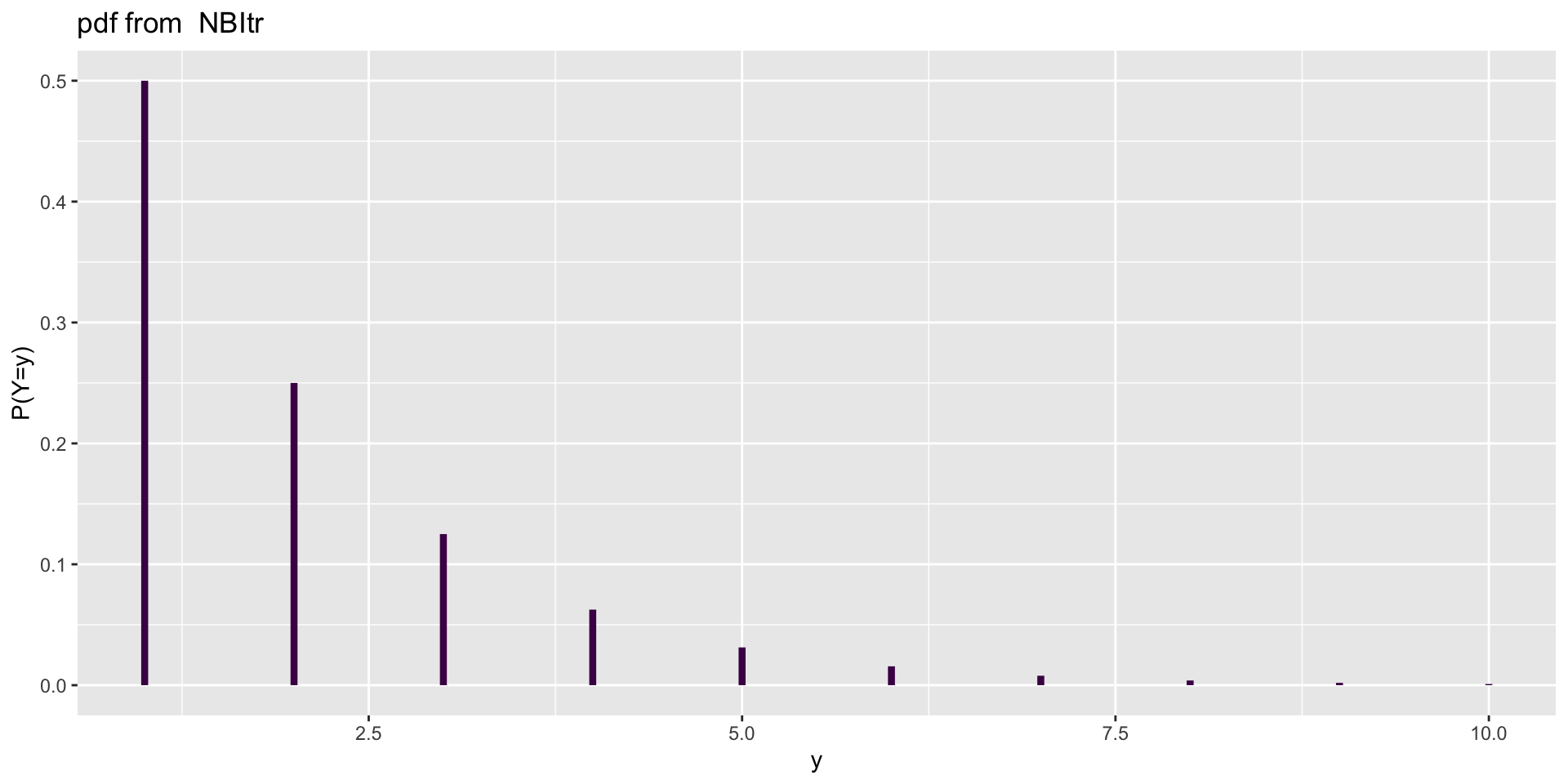
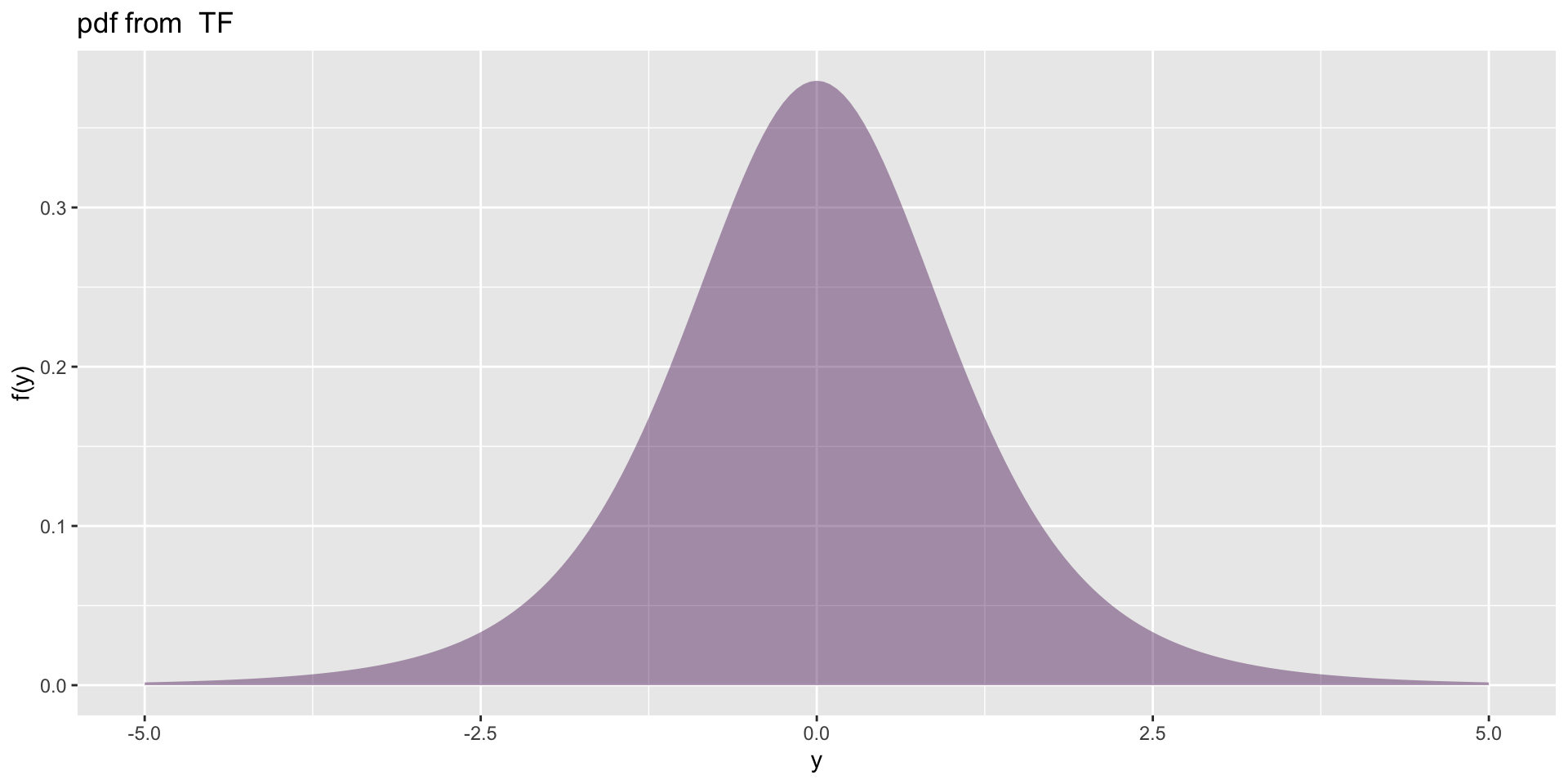
log distributions

log distributions (con)
A  log  family of distributions from TF has been generated
 and saved under the names:
dlogTF plogTF qlogTF rlogTF logTF 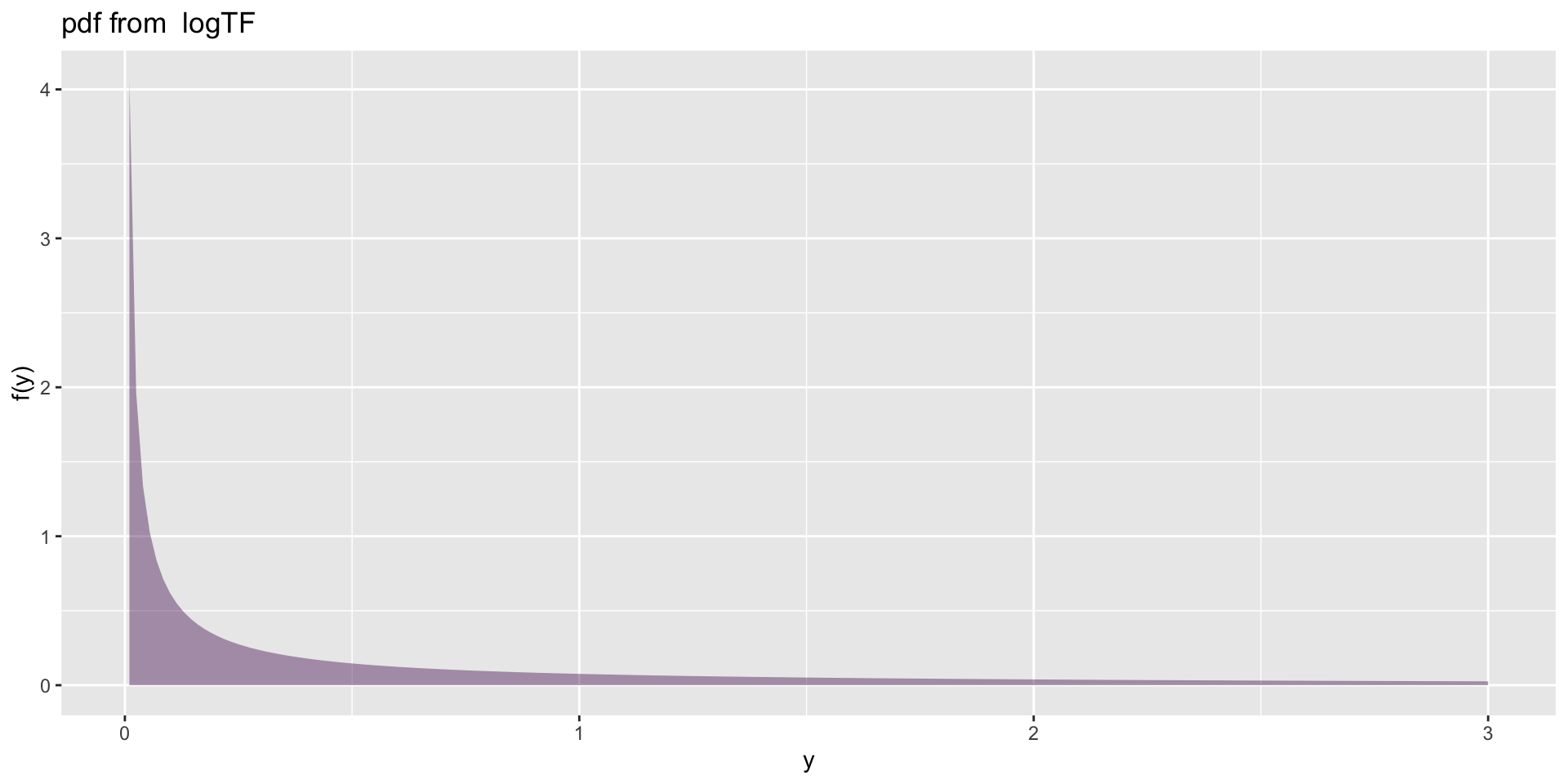
logit distributions
logit distributions (con)
A  logit  family of distributions from TF has been generated
 and saved under the names:
dlogitTF plogitTF qlogitTF rlogitTF logitTF 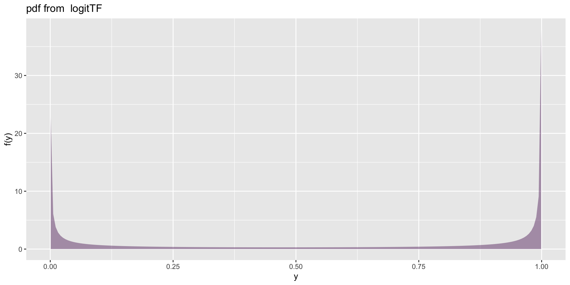
inflated distributions
A  logit  family of distributions from SHASHo has been generated
 and saved under the names:
 dlogitSHASHo plogitSHASHo qlogitSHASHo rlogitSHASHo logitSHASHo
A 0to1 inflated logitSHASHo distribution has been generated
and saved under the names:
dlogitSHASHoInf0to1 plogitSHASHoInf0to1 qlogitSHASHoInf0to1 rlogitSHASHoInf0to1
plotlogitSHASHoInf0to1 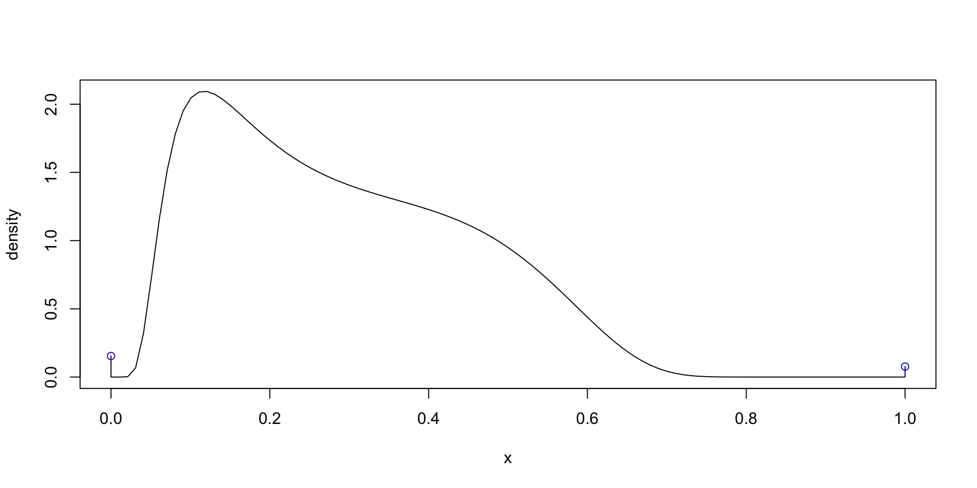
zero adjusted
A zero adjusted BCT distribution has been generated
 and saved under the names:
 dBCTZadj pBCTZadj qBCTZadj rBCTZadj
plotBCTZadj 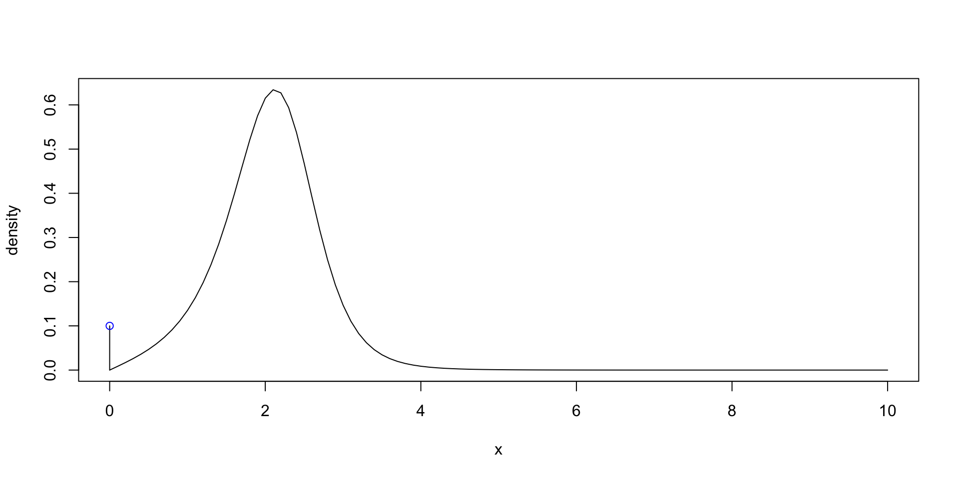
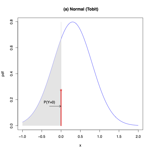
TOBIT
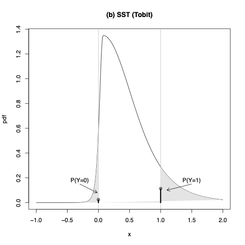
generalized TOBIT
book 2

book2
end
 The Books
![]()