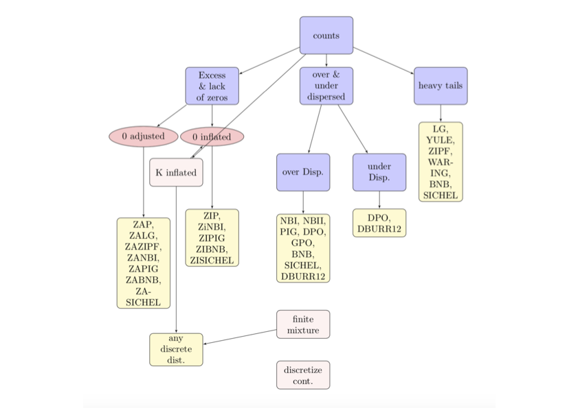
Discrete Distributions
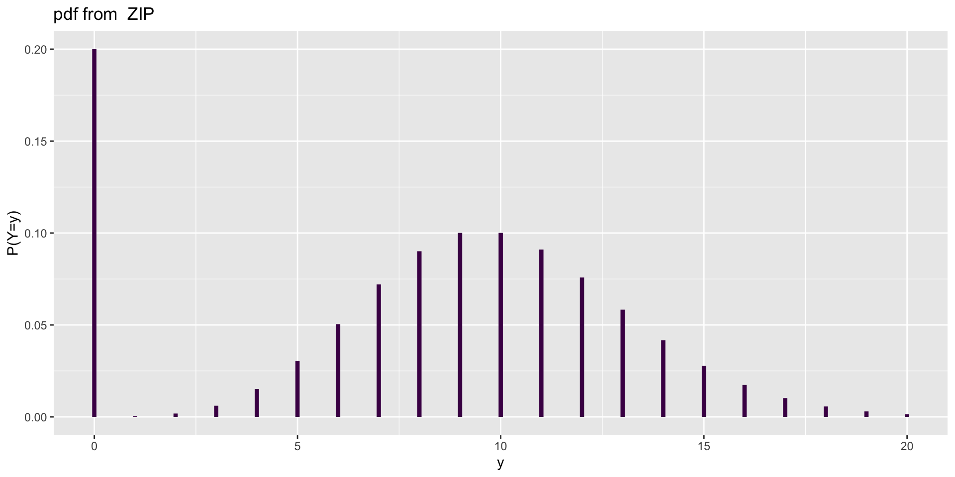
flow chart
Different types of count (NBI)

Different types of count (NBItr)
A truncated family of distributions from NBI has been generated
 and saved under the names:
 dNBItr pNBItr qNBItr rNBItr NBItr
The type of truncation is left
and the truncation parameter is 0 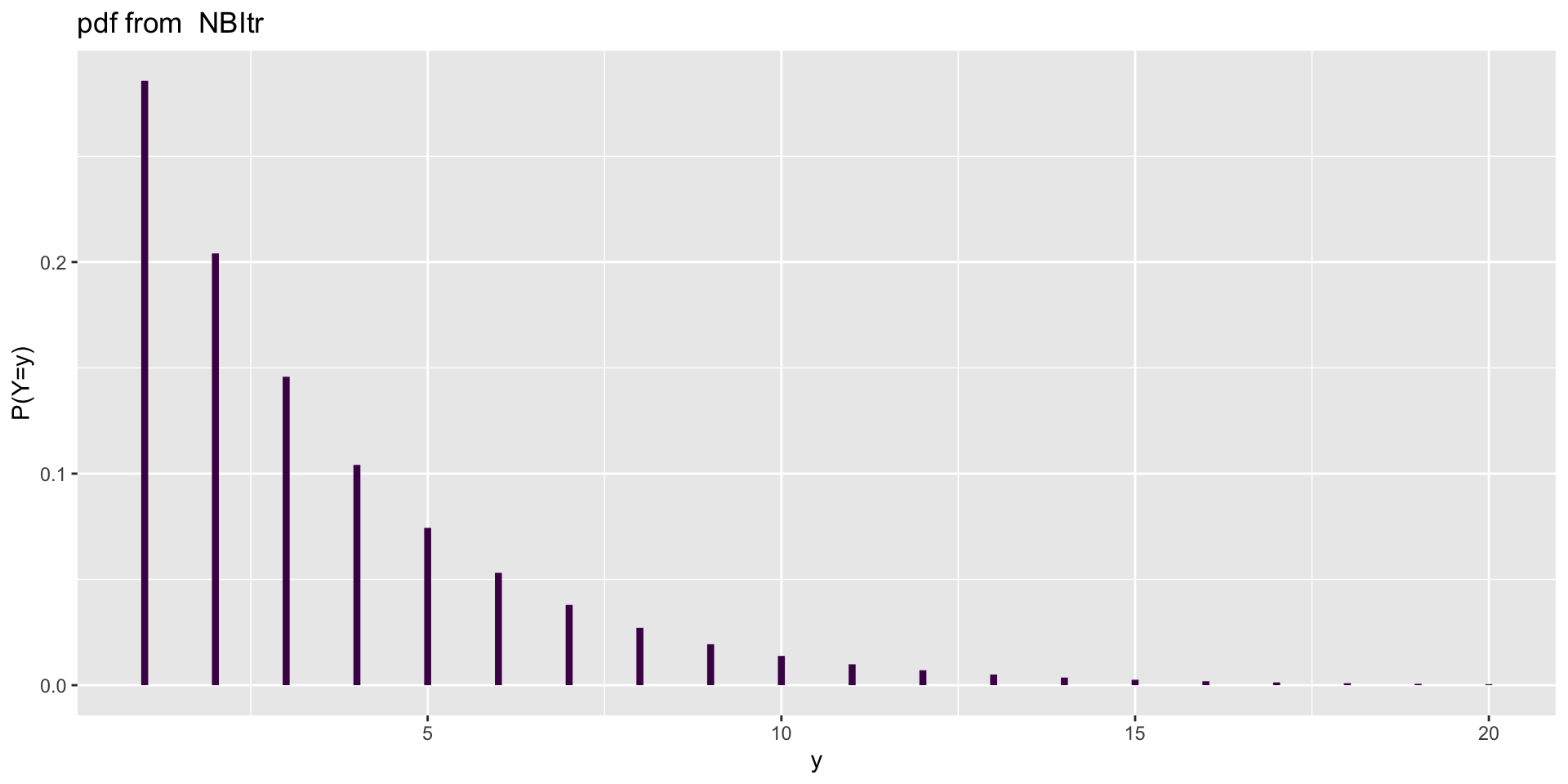
Different types of count (PIG)

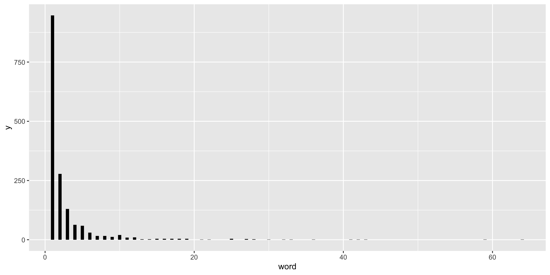
stylometric: plot (con.)
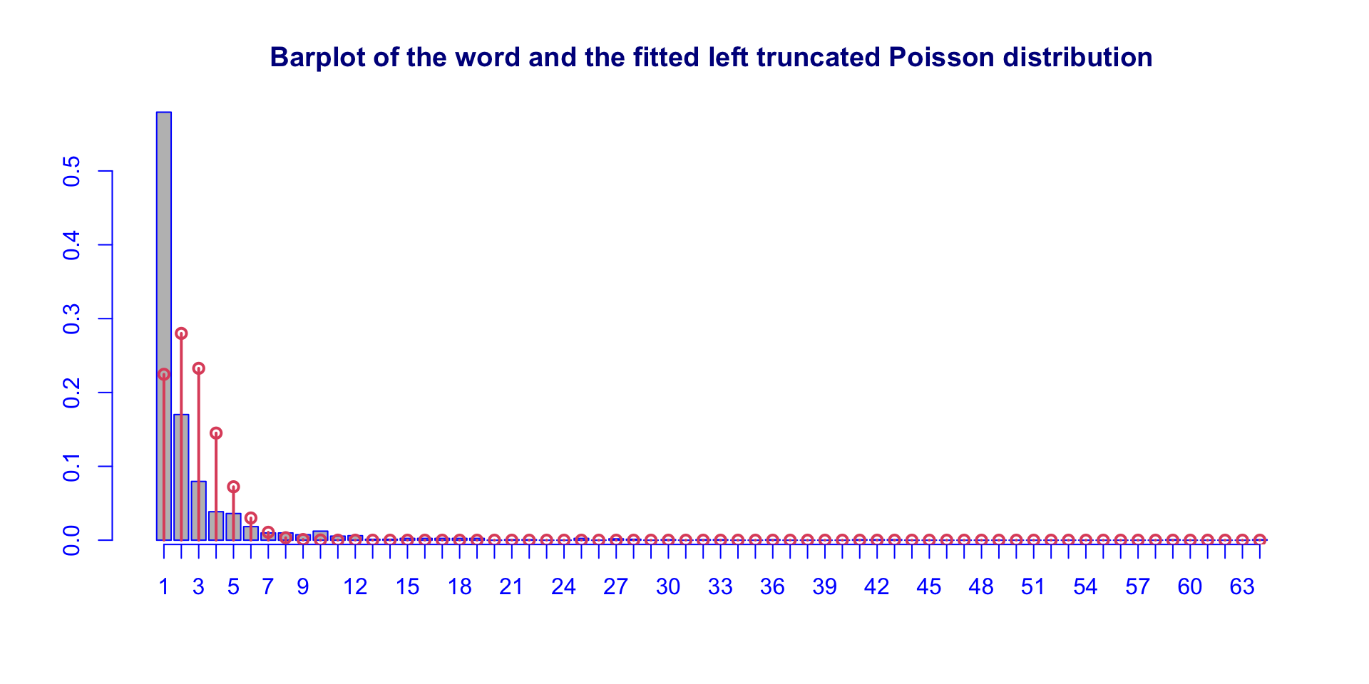
stylometric: fitted POtr (con.)
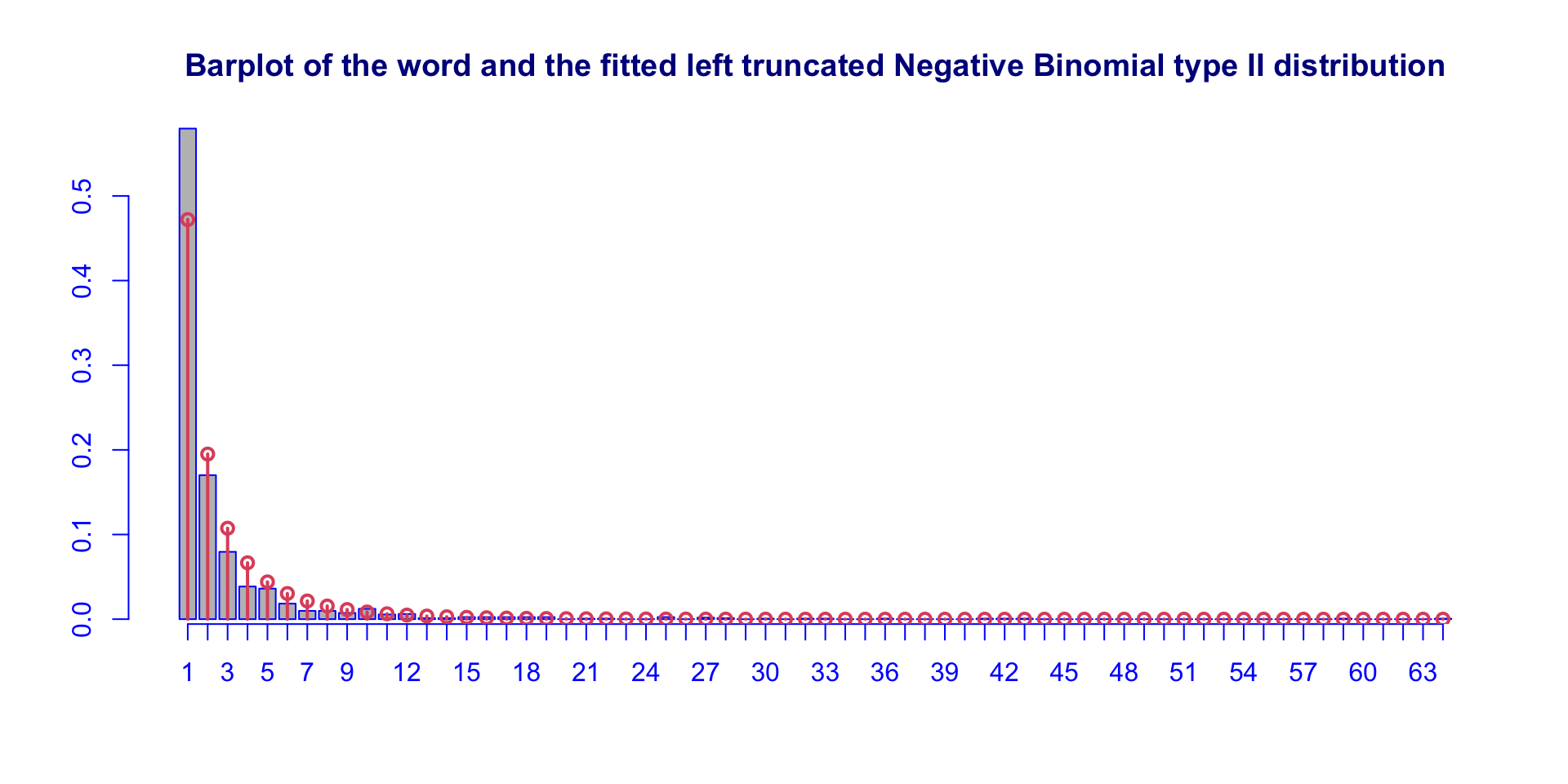
stylometric: fitted NBIItr (con.)
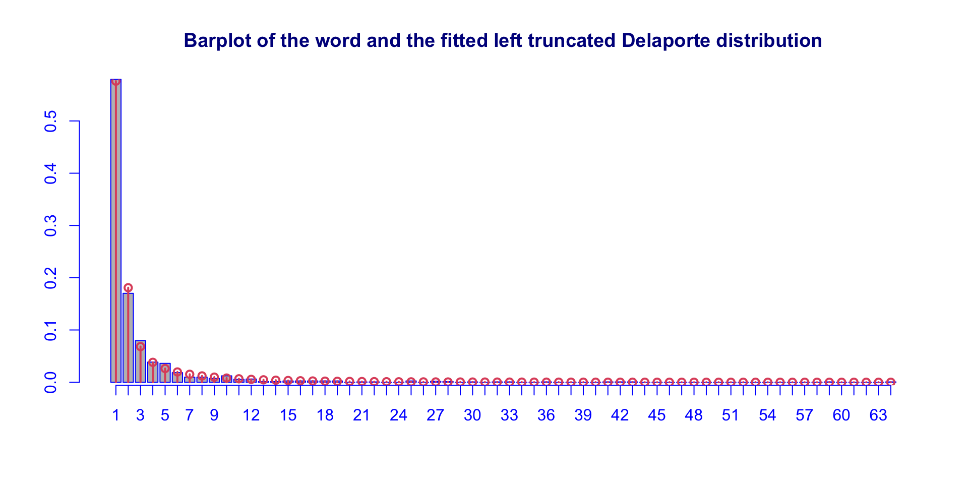
stylometric: fitted DELtr (con.)
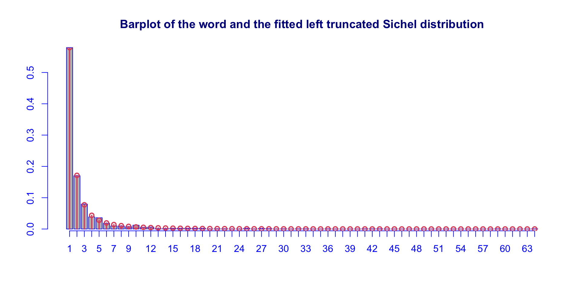
stylometric: fitted SICHELtr (con.)
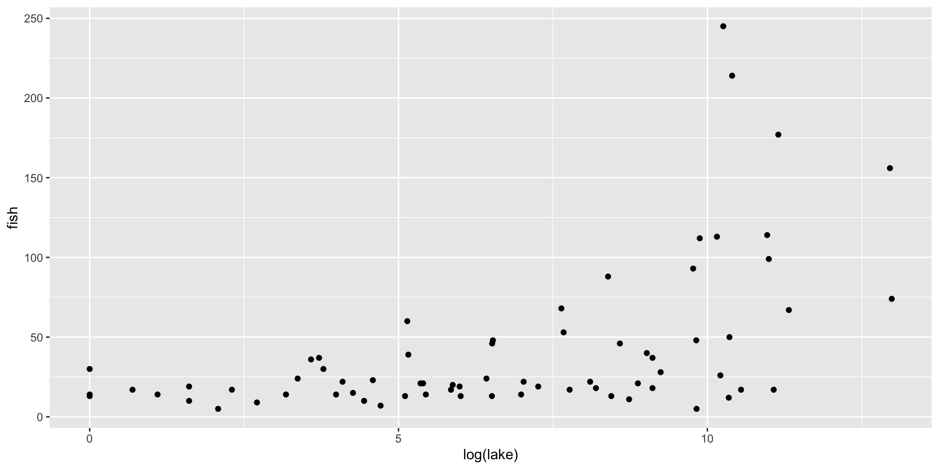
fish species plot
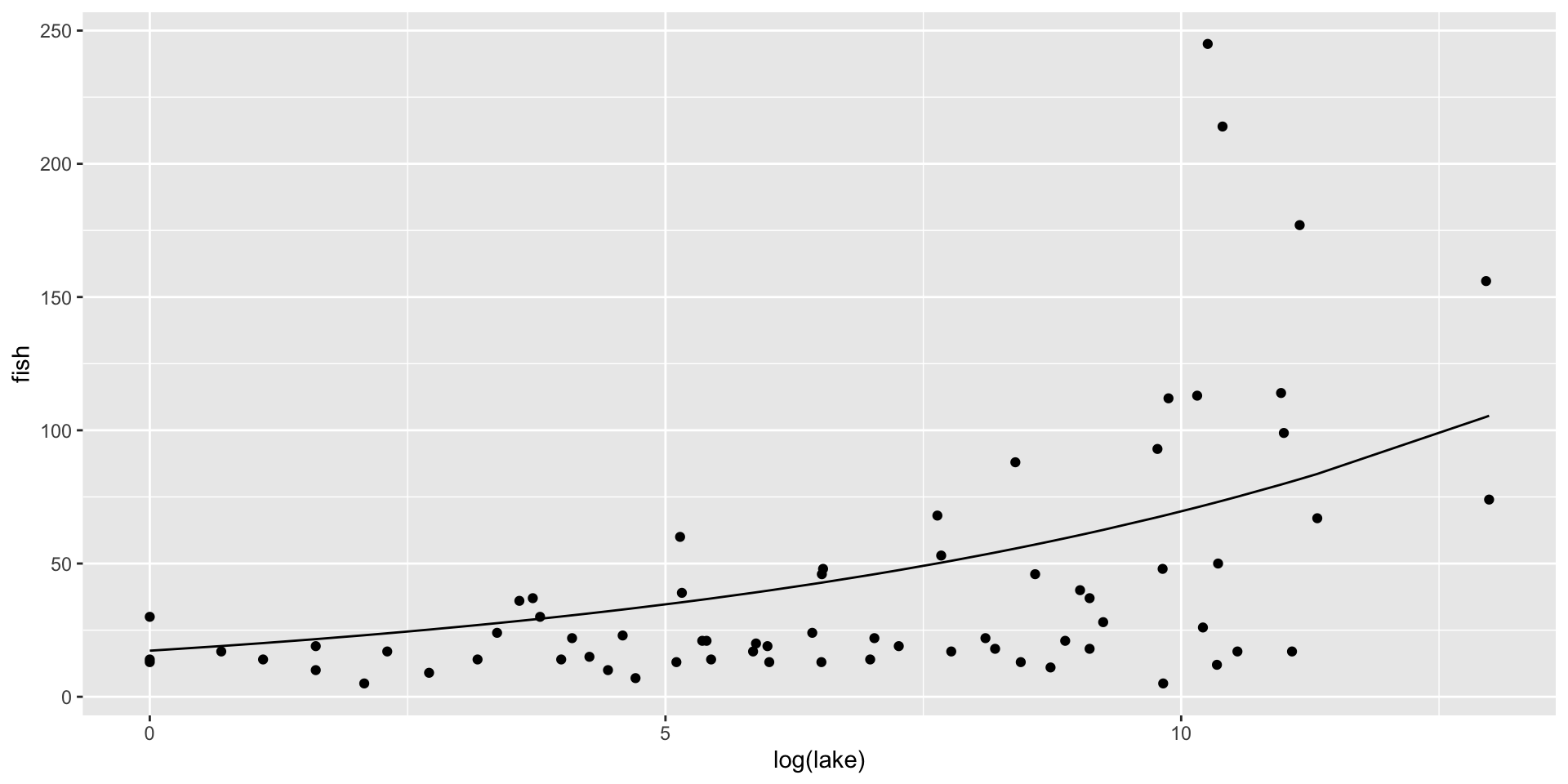
fish species fitted mean
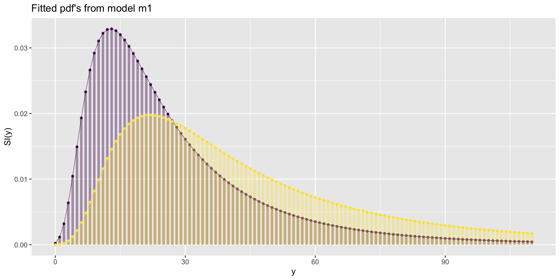
fish species fitted pdf
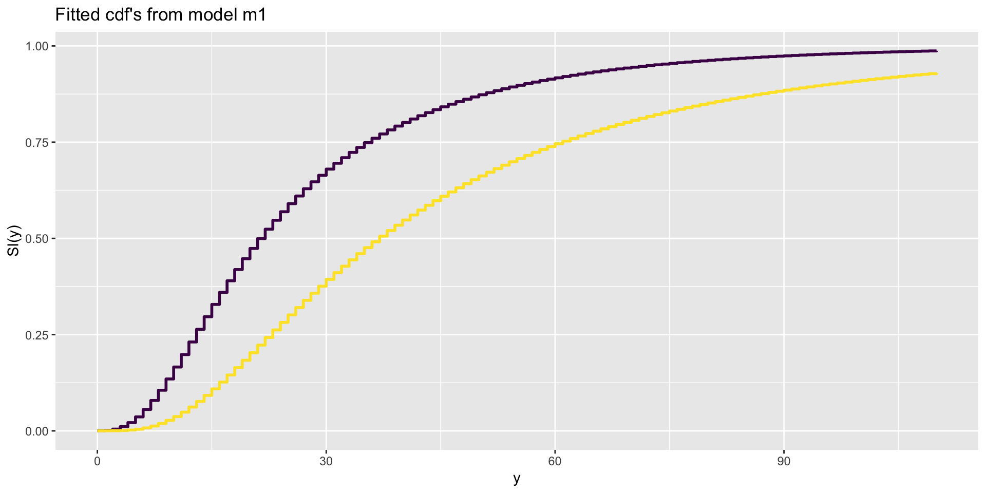
fish species fitted cdf
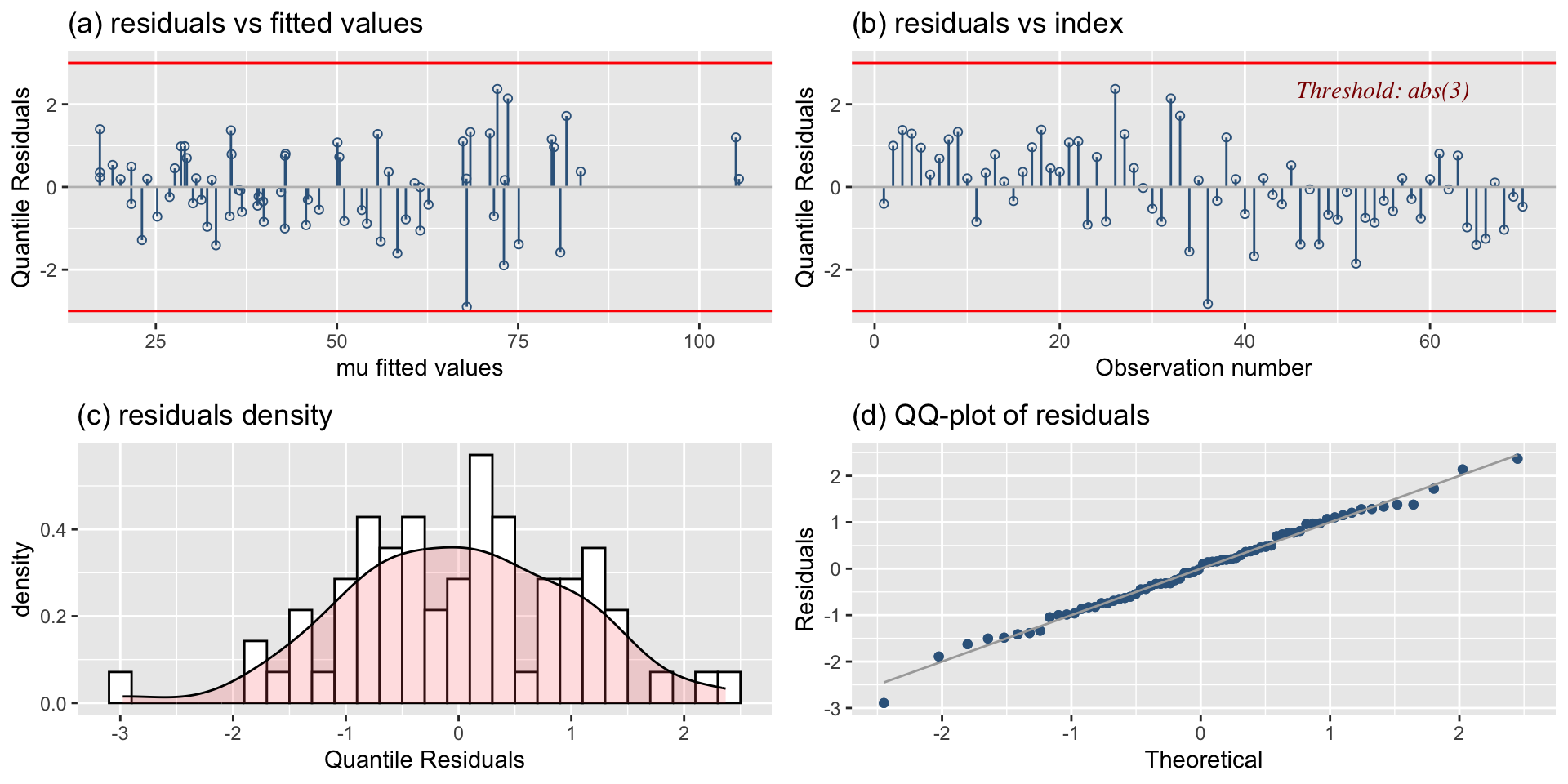
fish species diagnostics
the hospital stay data
library(gamlss.prepdata)
da <- aep[, -c(1,2,3,8,9)]
da$r <- with(aep, noinap/los*100)
data_xyplot(da, response=r)
100 % of data are ploted,
that is, 1383 observations. 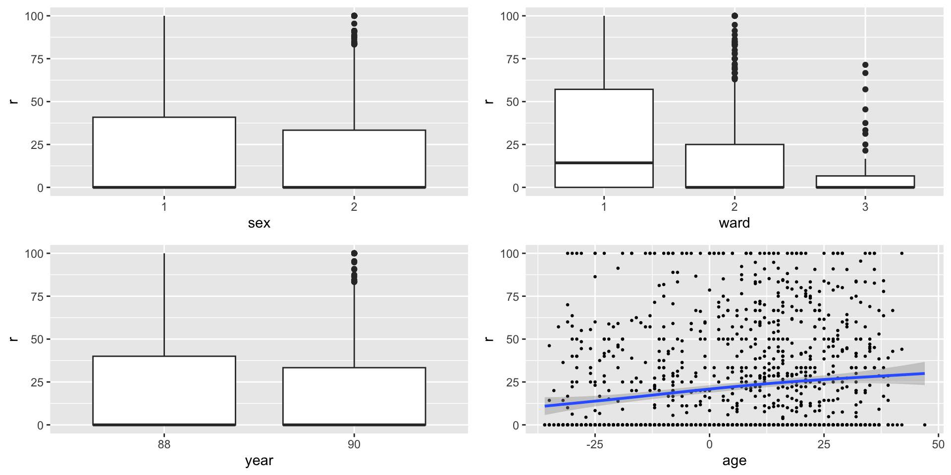
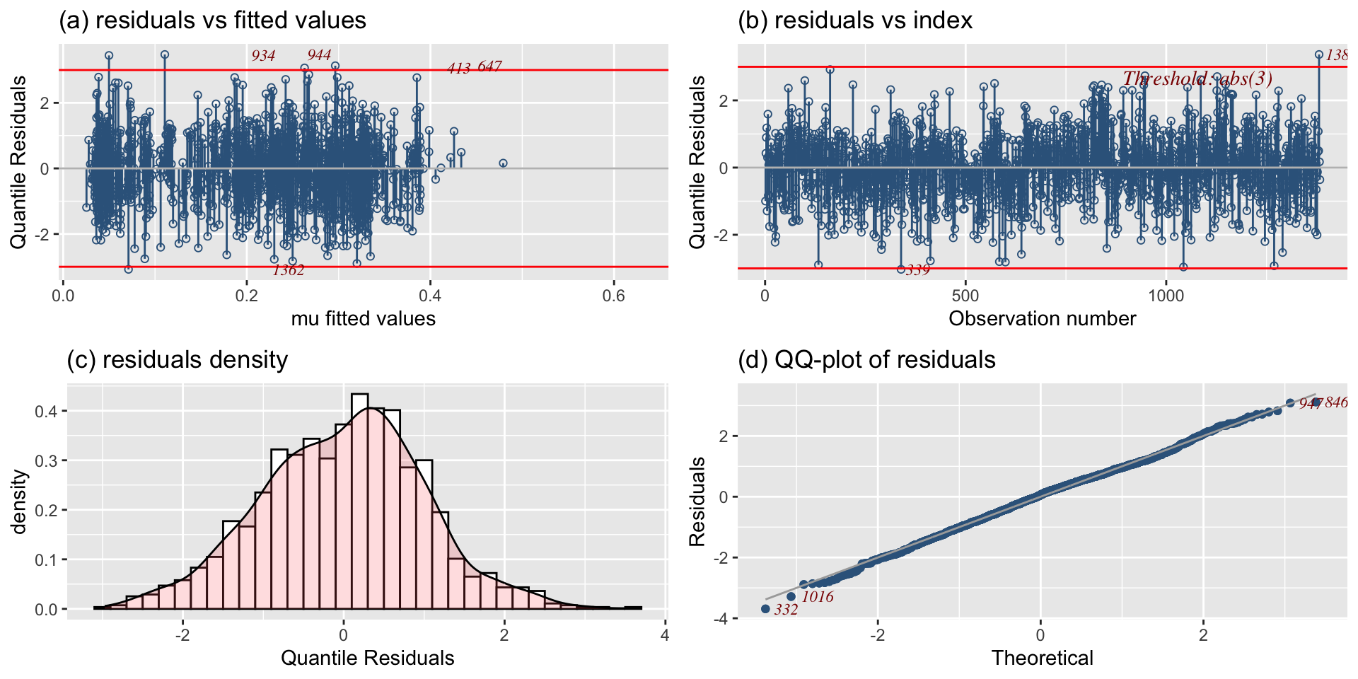
the hospital stay fits
END
 The Books
![]()