Continuous Distributions

Mikis Stasinopoulos

Bob Rigby

Gillian Heller

Fernanda De Bastiani

Niki Umlauf

Types

\((-\infty, \infty)\) real line \(\Re\) [Chapter 4 of Rigby et al (2019)]
\((0, \infty )\) positive real line \(\Re^{+}\) [Chapter 5]
\((0,1)\) real line on interval \(\Re_{(0,1)}\) (not containing zero or one) [Chapter 6]

Explicit distributions in real line, \(\Re\).

`Location` and `Scale` family

if \[Y\sim {D}(\mu,\sigma,\nu,\tau)\] then \[\varepsilon=(Y-\mu)/\sigma\sim {D}(0,1,\nu,\tau),\]

i.e. \(Y=\mu+\sigma\varepsilon\), so \(Y\) is a scaled and shifted version of the random variable \(\varepsilon\).

location

scale

2 parameter in \(\Re\)

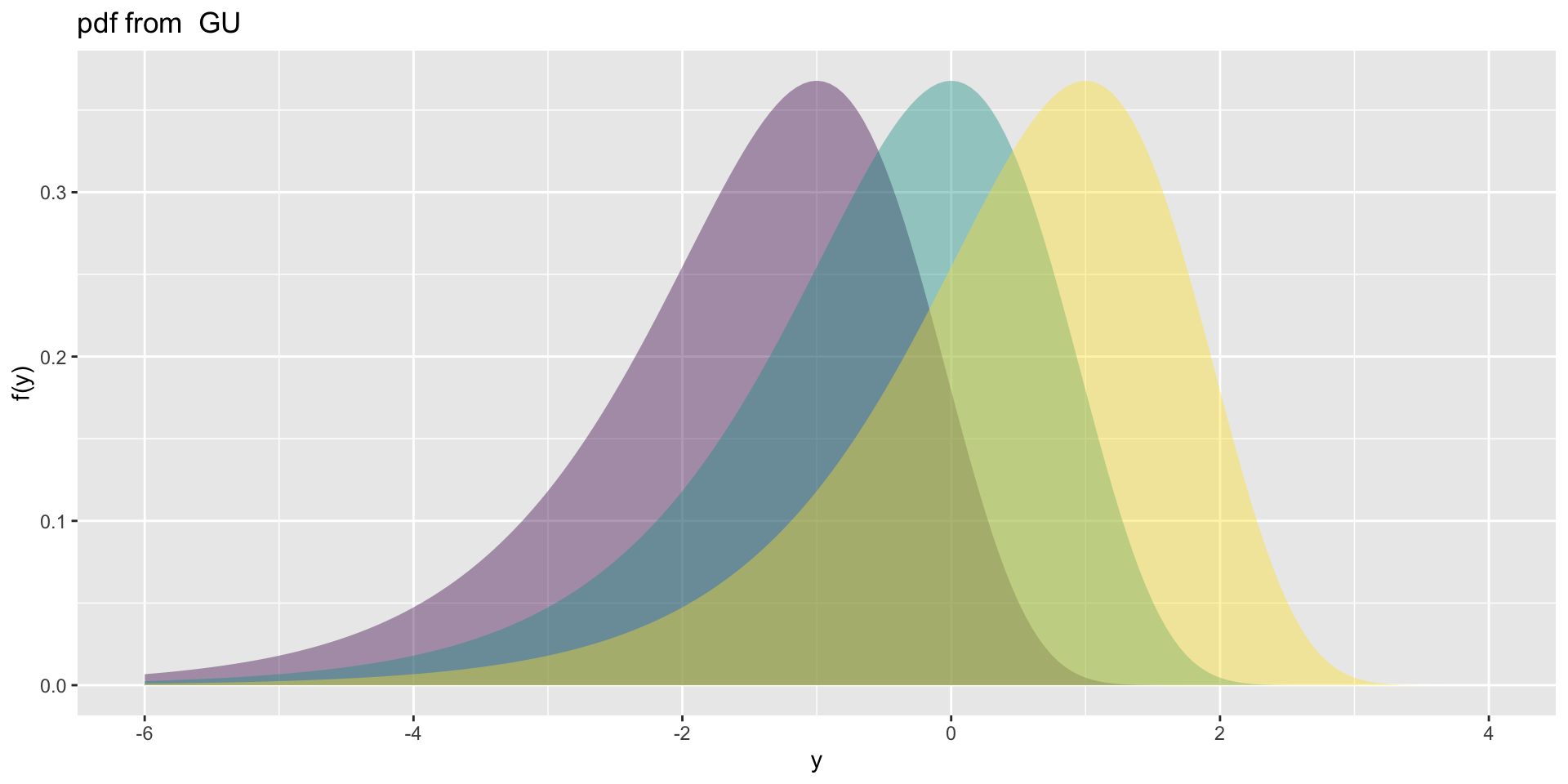
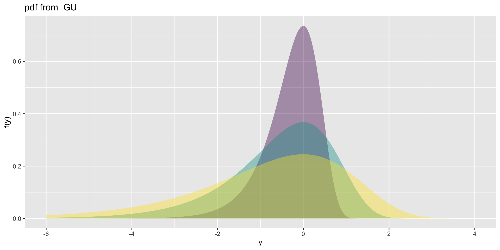
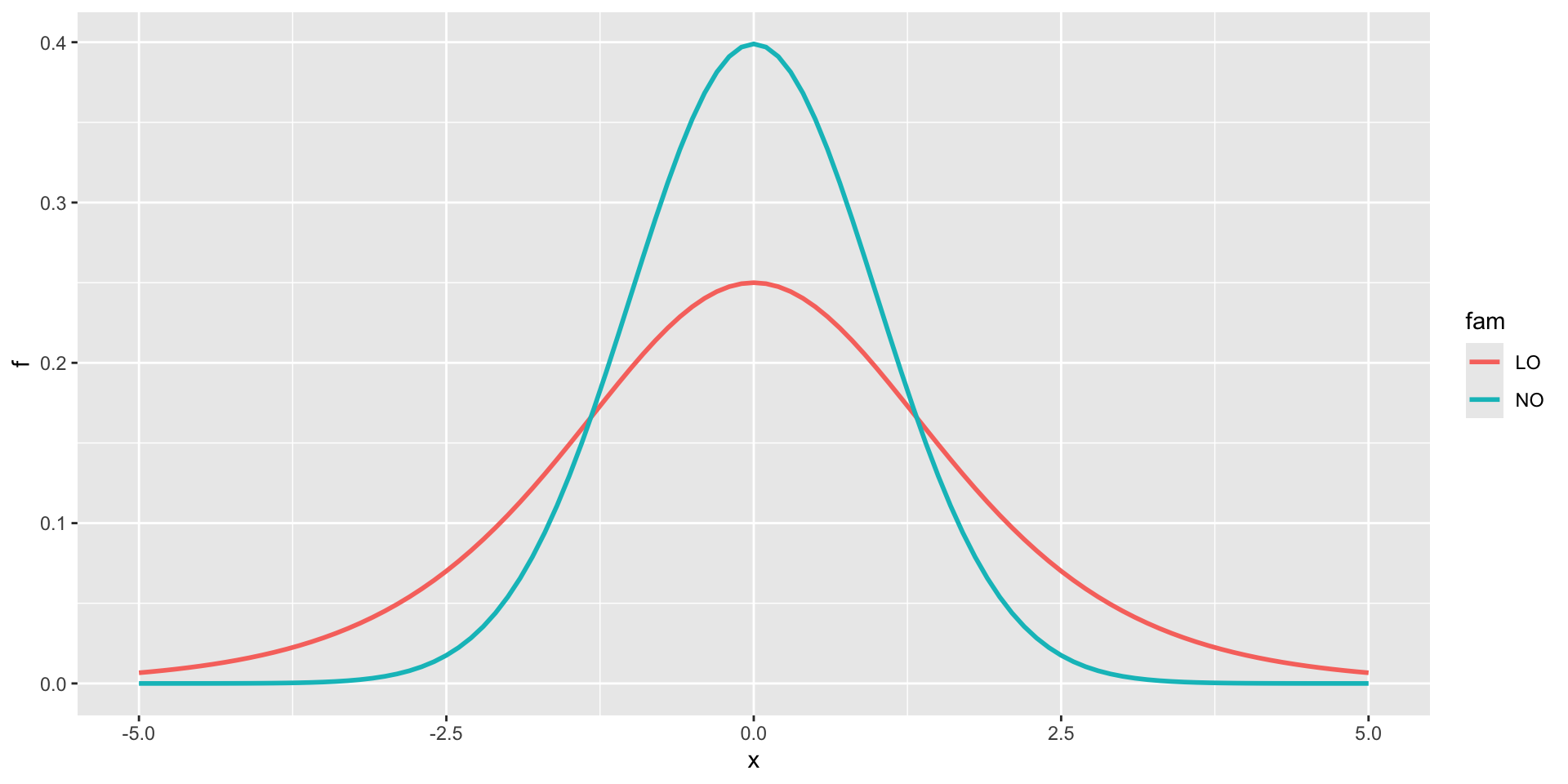
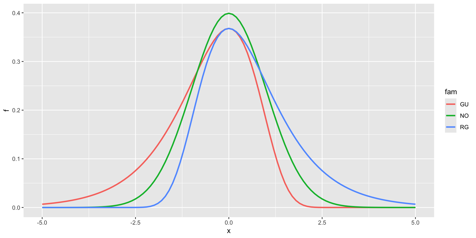
Gumbel, GU(\(\mu\), \(\sigma\)), left skew
Logistic, LO(\(\mu\), \(\sigma\)), lepto
Normal, NO(\(\mu\), \(\sigma\)), NO(\(\mu\), \(\sigma^2\))
Reverse Gumbel RG(\(\mu\), \(\sigma\)), right skew

2 parameter in \(\Re\) (con.)

Normal against Logistic

2 parameter in \(\Re\) (con.)

Normal against Gumbel and reverse Gumbel

3 parameter in \(\Re\)

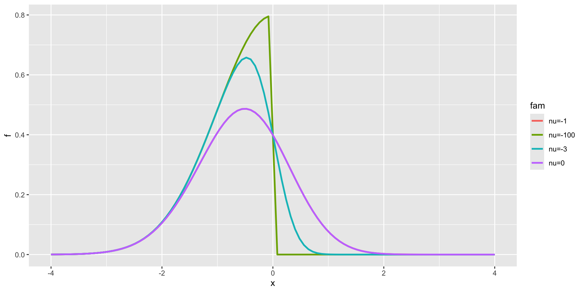
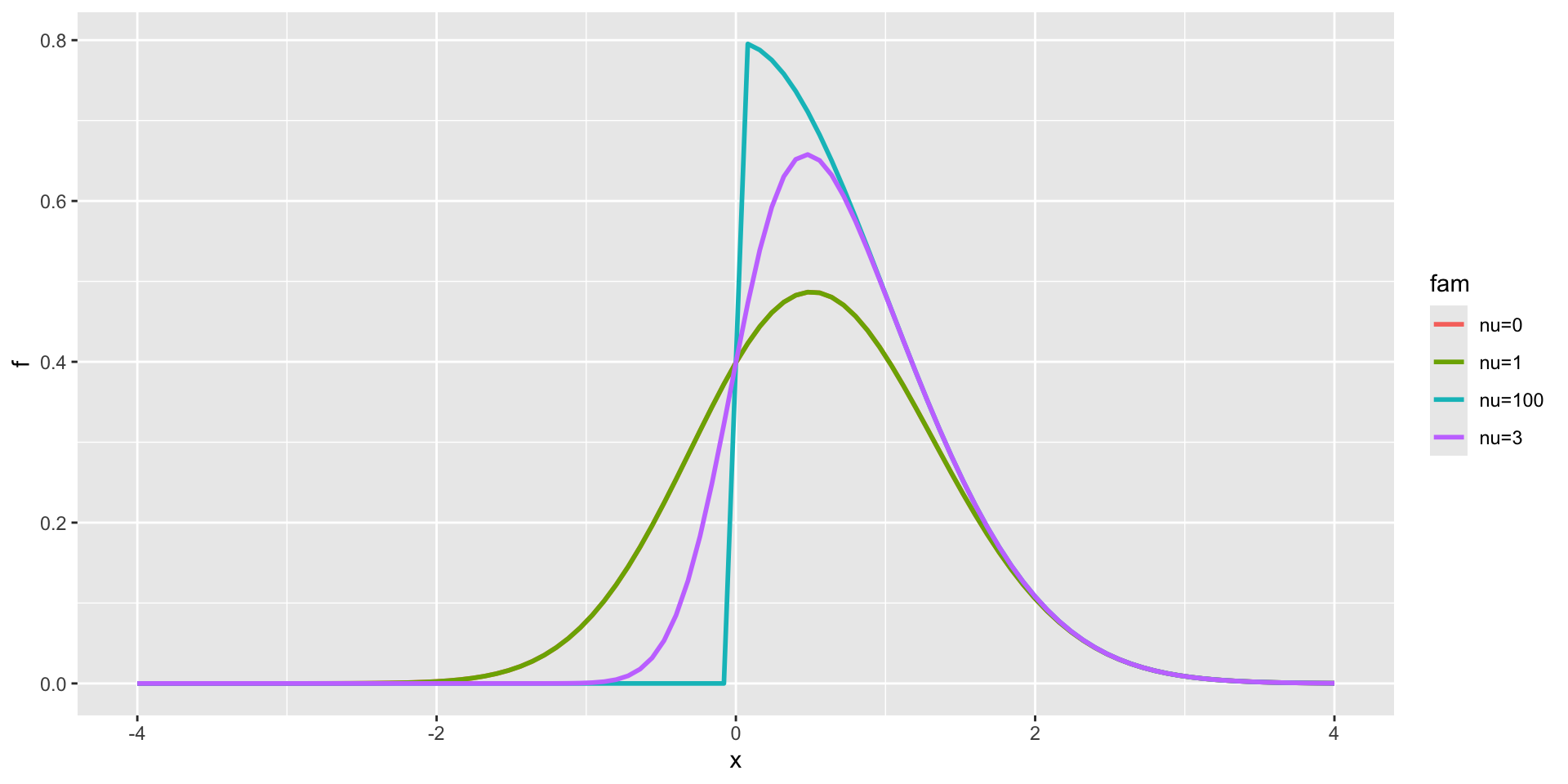
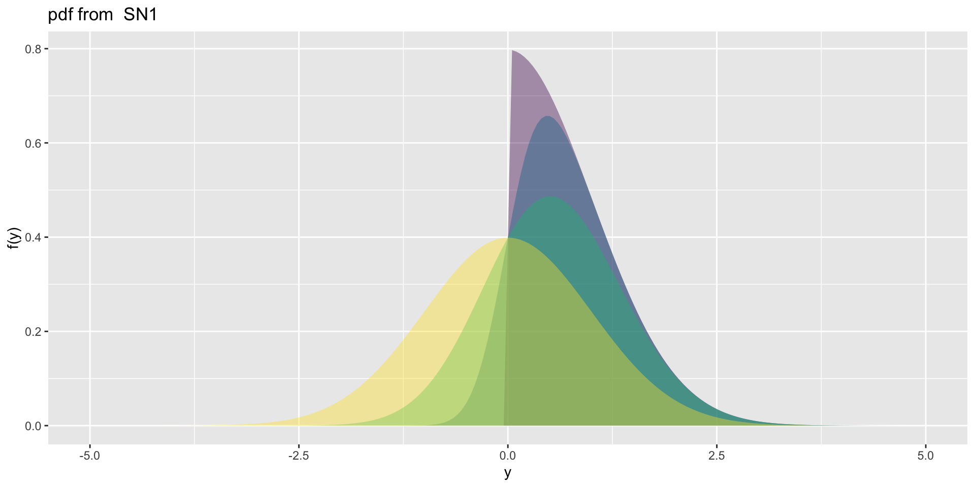
exponential Gaussian: exGAUS\((\mu, \sigma, \nu)\) for modelling right skew data,
normal family: NOF\((\mu, \sigma, \nu)\) for modelling mean and variance relationships following the power law;
power exponential: PE\((\mu, \sigma, \nu)\) and PE2\((\mu, \sigma, \nu)\) for modelling lepto and platy kurtotic data;
t family: TF\((\mu, \sigma, \nu)\) and TF2\((\mu, \sigma, \nu)\) for modelling lepro kurtotic data;
skew normal: SN1\((\mu, \sigma, \nu)\) and SK2\((\mu, \sigma, \nu)\) for modellinng skewness in data.

3 parameter in \(\Re\) (con.)

Skew Normal type 1

3 parameter in \(\Re\) (con.)

Skew Normal type 1

3 parameter in \(\Re\) (TEST 1)

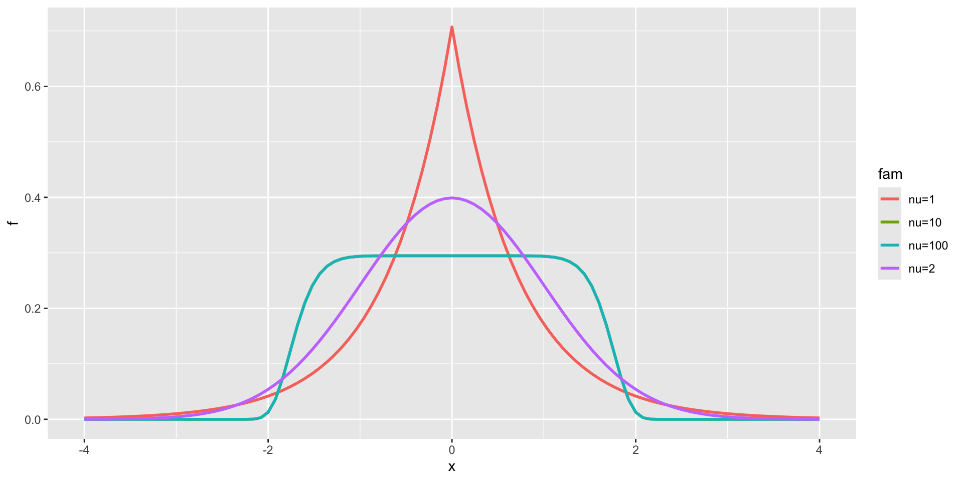
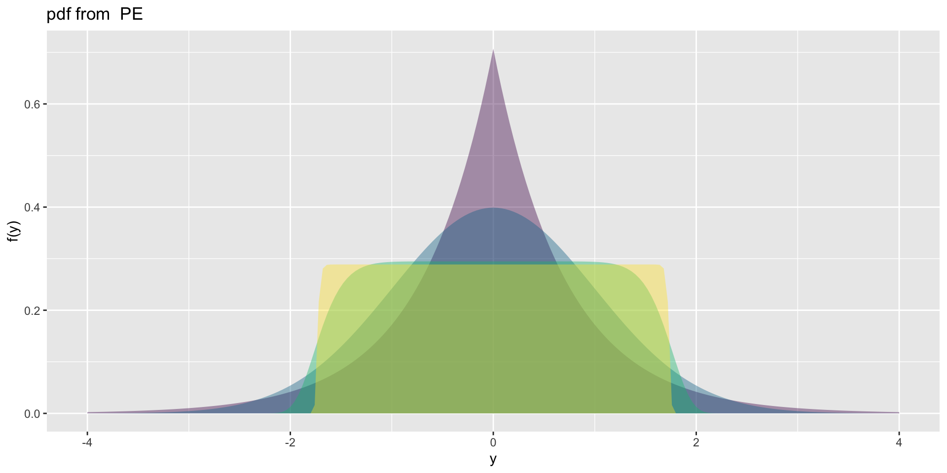
3 parameter in \(\Re\) PE

Power Exponential

3 parameter in \(\Re\) PE (test)

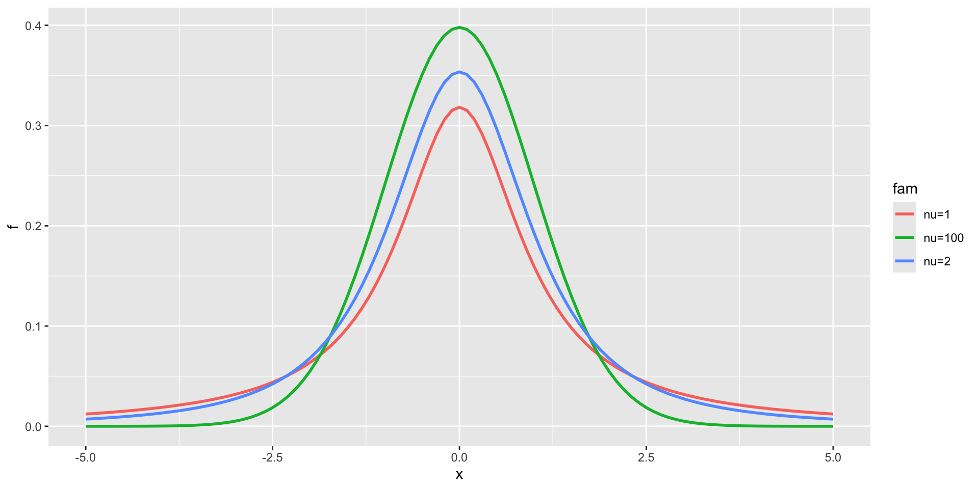
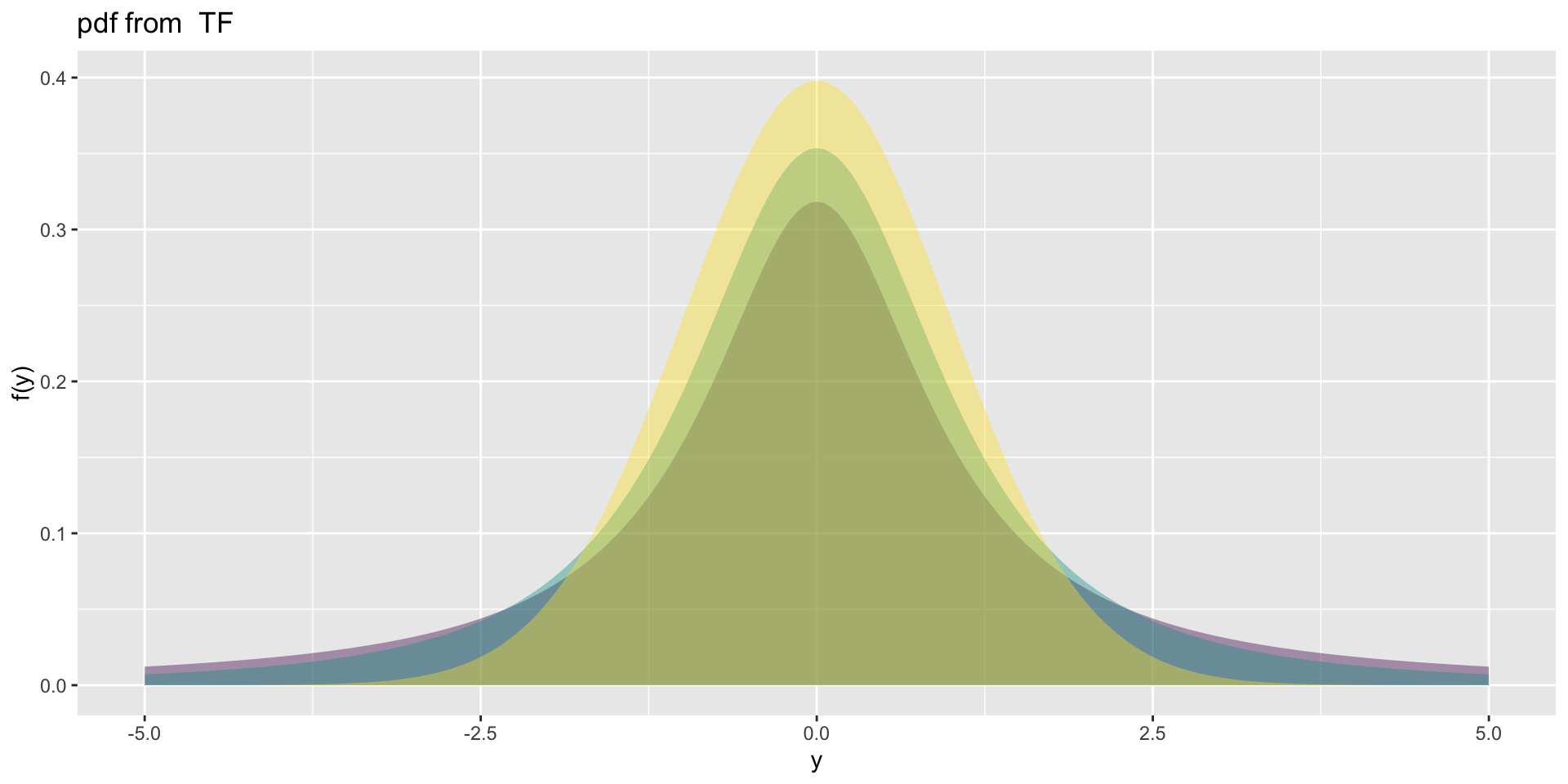
3 parameter in \(\Re\) TF

t family

3 parameter in \(\Re\) TF (test)

4 parameter in \(\Re\)

exponential generalised beta type 2,
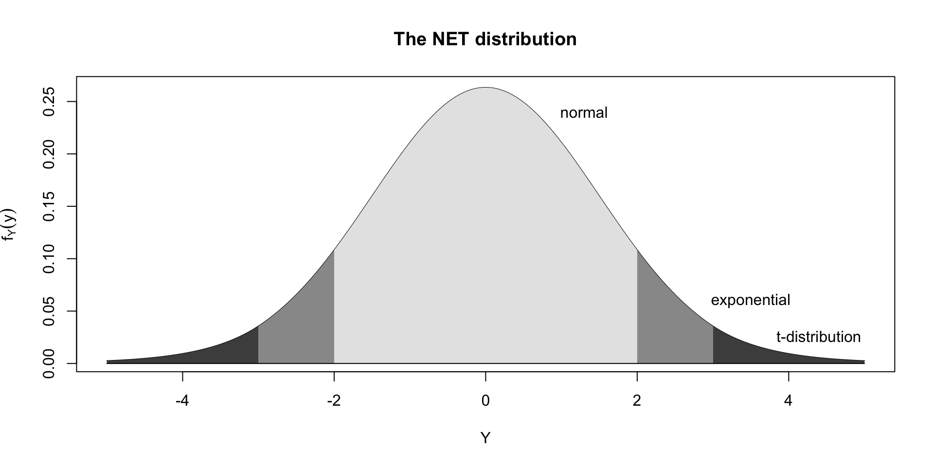
\(EGB2(\mu,\sigma,\nu,\tau)\) skewness and leptokurtosis;
generalised t, GT\((\mu,\sigma, \nu, \tau)\) kurtosis;
Johnson's SU, JSU\((\mu,\sigma, \nu, \tau)\) and \(\texttt{JSUo}(\mu,\sigma, \nu, \tau)\) skewness and leptokurtosis;
normal-exponential-t \(\texttt{NET}(\mu,\sigma, \nu, \tau)\), robustly location and scale
skew exponential power \(\texttt{SEP1}(\mu,\sigma, \nu, \tau)\), \(\texttt{SEP2}(\mu,\sigma, \nu, \tau)\), \(\texttt{SEP3}(\mu,\sigma, \nu, \tau)\) and \(\texttt{SEP4}(\mu,\sigma, \nu, \tau)\) skewness and lepto-platy;

4 parameter in \(\Re\) (con.)

sinh-arcsinh, \(\texttt{SHASH}(\mu,\sigma, \nu, \tau)\), \(\texttt{SHASHo}(\mu,\sigma, \nu, \tau)\) and \(\texttt{SHASHo2}(\mu,\sigma, \nu, \tau)\) skewness and lepto-platy;
skew t, \(\texttt{ST1}(\mu,\sigma, \nu, \tau)\), \(\texttt{ST2}(\mu,\sigma, \nu, \tau)\), \(\texttt{ST3}(\mu,\sigma, \nu, \tau)\), \(\texttt{ST4}(\mu,\sigma, \nu, \tau)\), \(\texttt{ST5}(\mu,\sigma, \nu, \tau)\) and \(\texttt{SST}(\mu,\sigma, \nu, \tau)\) skewness and leptokurtosis.

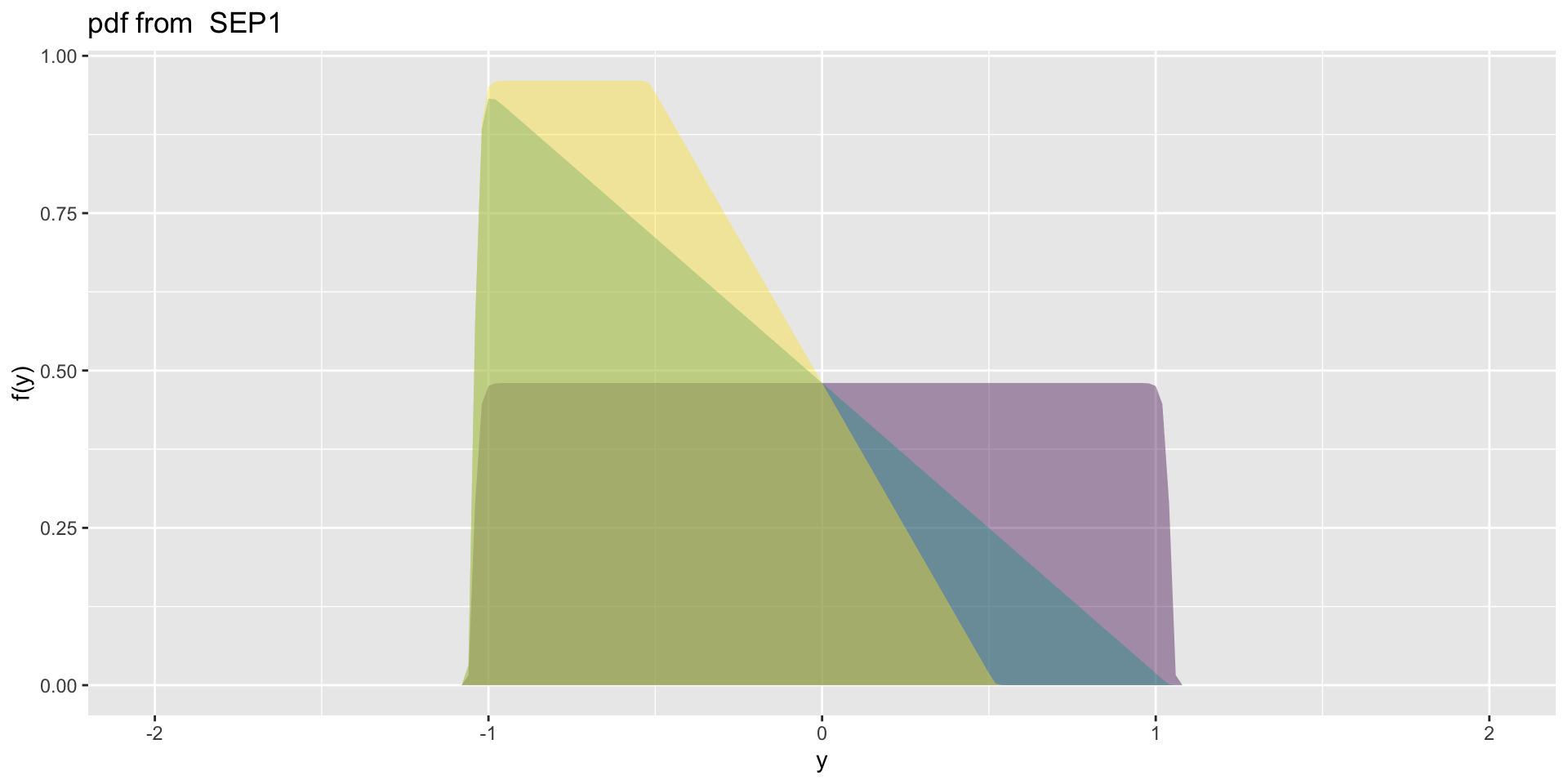
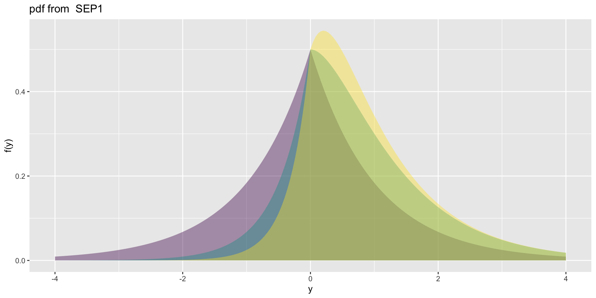
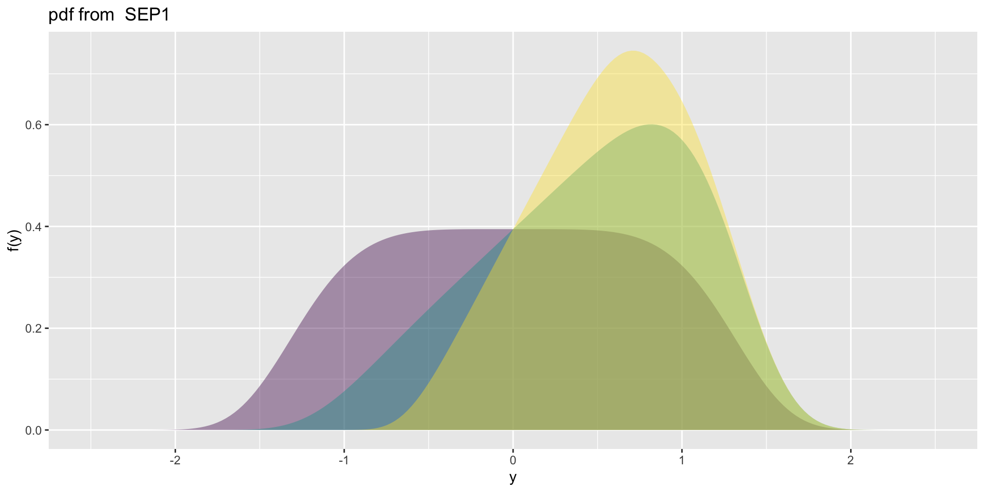
4 parameter in \(\Re\) SEP1

SEP1\(\mu=0, \sigma=1, \nu=0,1,2, \tau=1\)

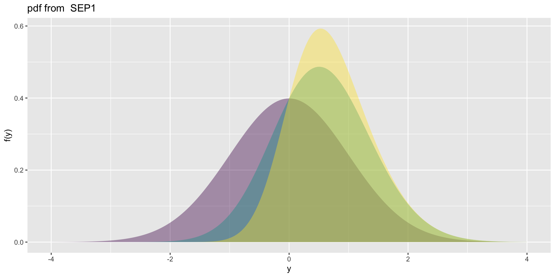
4 parameter in \(\Re\) SEP1

SEP1\(\mu=0, \sigma=1, \nu=0,1,2, \tau=2\)

4 parameter in \(\Re\) SEP1

SEP1\(\mu=0, \sigma=1, \nu=0,1,2, \tau=5\)

4 parameter in \(\Re\) SEP1

4 parameter in \(\Re\) NET

Summary

Distributions	family	no par.	skewness	kurtosis
Exp. Gaussian	exGAUS	3	positive	-
Exp.G. beta 2	EGB2	4	both	lepto
Gen. t	GT	4	(symmetric)	lepto
Gumbel	GU	2	(negative)	-
Johnson’s SU	JSU, JSUo	4	both	lepto
Logistic	LO	2	(symmetric)	(lepto)
Normal-Expon.-t	NET	2,(2)	(symmetric)	lepto
Normal	NO-NO2	2	(symmetric)	(meso)
Normal Family	NOF	3	(symmetric)	(meso)
Power Expon.	PE-PE2	3	(symmetric)	both
Reverse Gumbel	RG	2	positive
Sinh Arcsinh	SHASH,	4	both	both
Skew Exp. Power	SEP1-SEP4	4	both	both
Skew t	ST1-ST5, SST	4	both	lepto
t Family	TF	3	(symmetric) lepto

Explicit Distributions in positive real line \(\Re^+\)

the scale family

If a random variable is distributed as \[Y\sim D(\mu,\sigma,\nu,\tau)\]

and
\[\varepsilon=(Y/\mu) \sim D(1,\sigma,\nu,\tau)\] then \(Y\) has a scale family

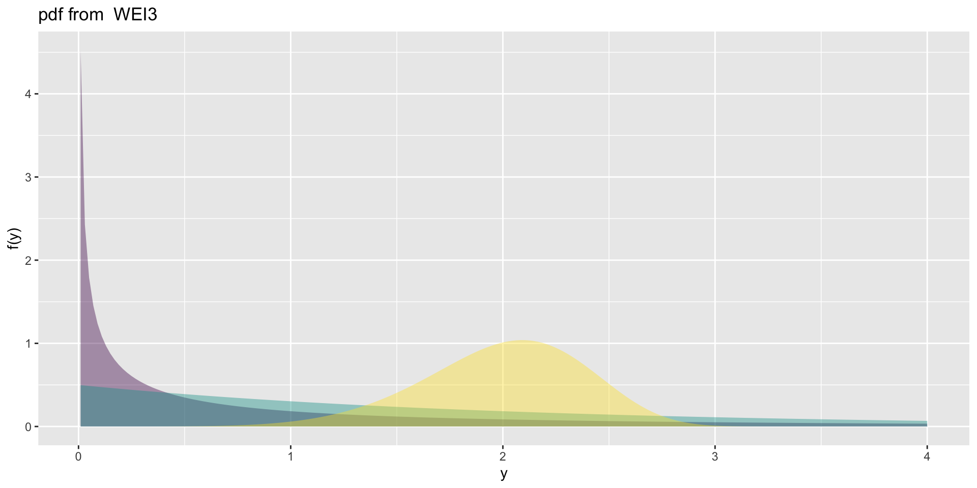
the weibull 3

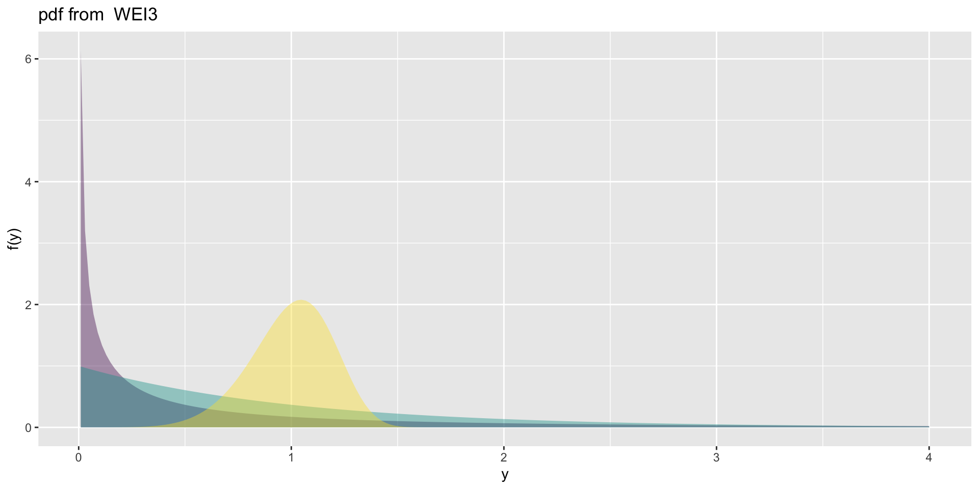
the weibull 3 (con.)

1 and 2 parameter positive real line, \(\Re^+\).

exponencial, \(\texttt{EXP}(\mu,\sigma)\)
gamma \(\texttt{GA}(\mu,\sigma)\) member of the exponential family;
inverse gamma \(\texttt{IGAMMA}(\mu,\sigma)\);
inverse Gaussian, \(\texttt{IG}(\mu,\sigma)\) a member of the exponential family;
log-normal \(\texttt{LOGNO}(\mu,\sigma)\) and \(\texttt{LOGNO2}(\mu,\sigma)\).
Pareto \(\texttt{PARETO}(\mu,\sigma)\), \(\texttt{PARETO2o}(\mu,\sigma)\) and \(\texttt{GP}(\mu,\sigma)\) for heavy tail;
Weibull \(\texttt{WEI}(\mu,\sigma)\), \(\texttt{WEI2}(\mu,\sigma)\) and \(\texttt{WEI3}(\mu,\sigma)\) used in survival analysis.

Weibull survival and hazard

3 parameter positive real line \(\Re^+\)

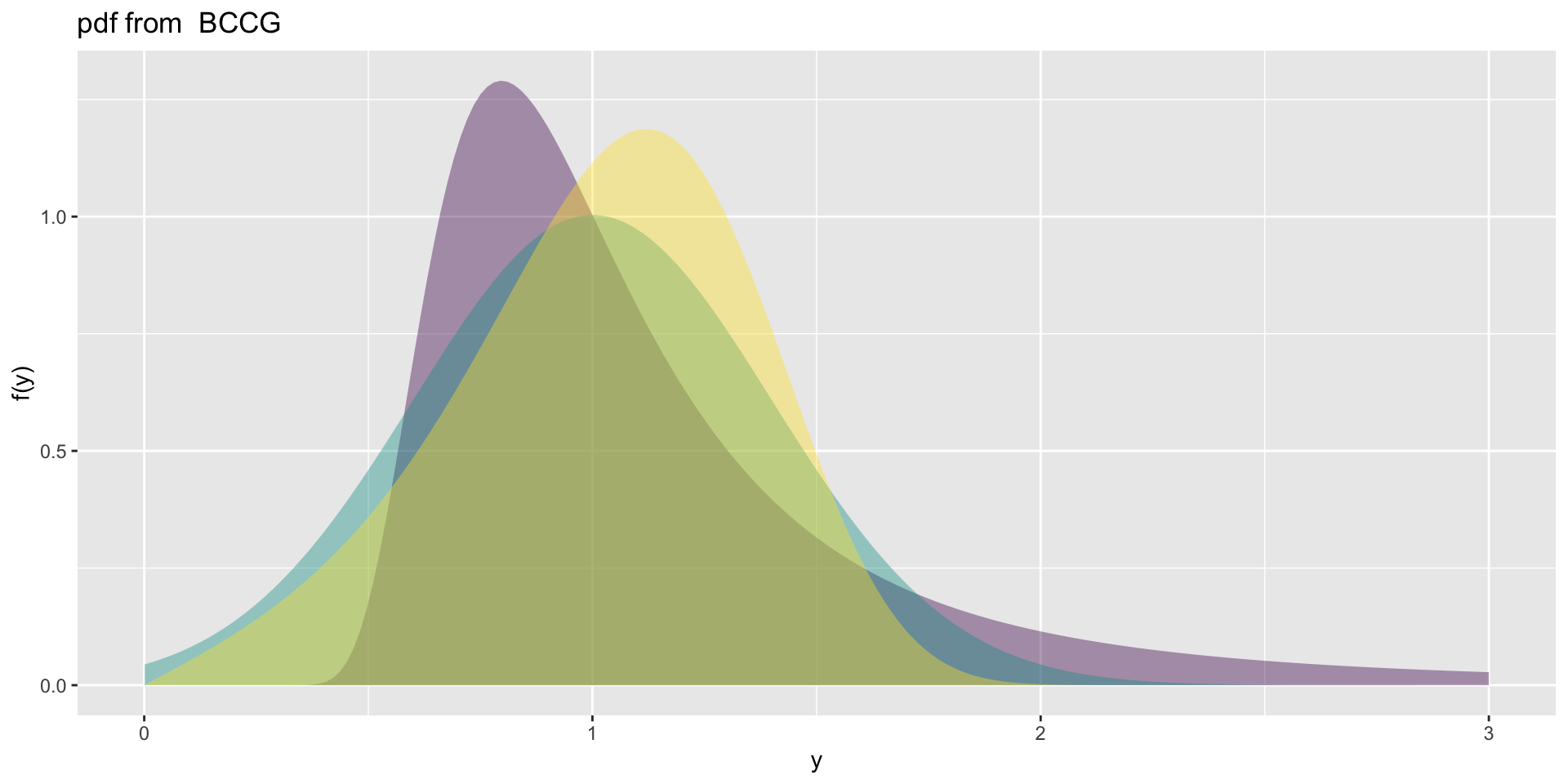
Box-Cox Cole and Green, \(\texttt{BCCG}(\mu, \sigma, \nu)\) known also as the LMS method in centile estimation.
generalised gamma, \(\texttt{GG}(\mu, \sigma, \nu)\)
generalised inverse Gaussian, \(\texttt{GIG}(\mu, \sigma, \nu)\)
log-normal family, \(\texttt{LNO}(\mu, \sigma, \nu)\) based on the standard Box-Cox transformation

the BCCG

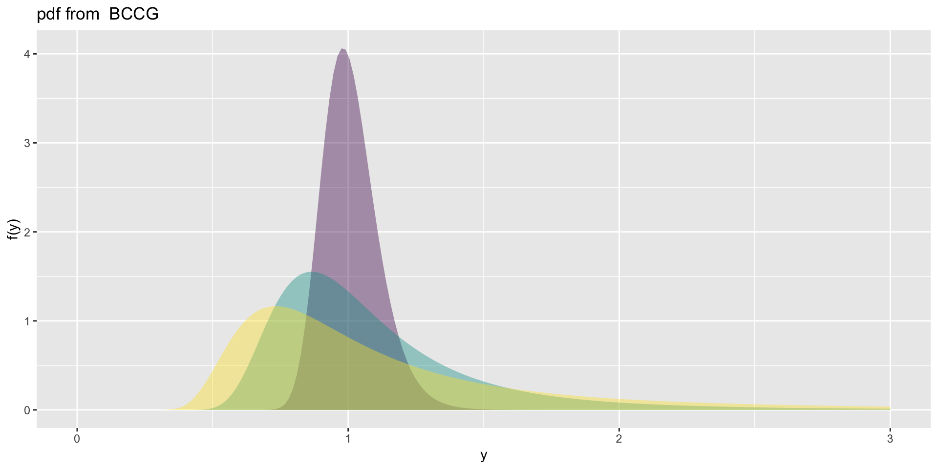
the BCCG (con.)

4 parameter positive real line \(\Re^+\)

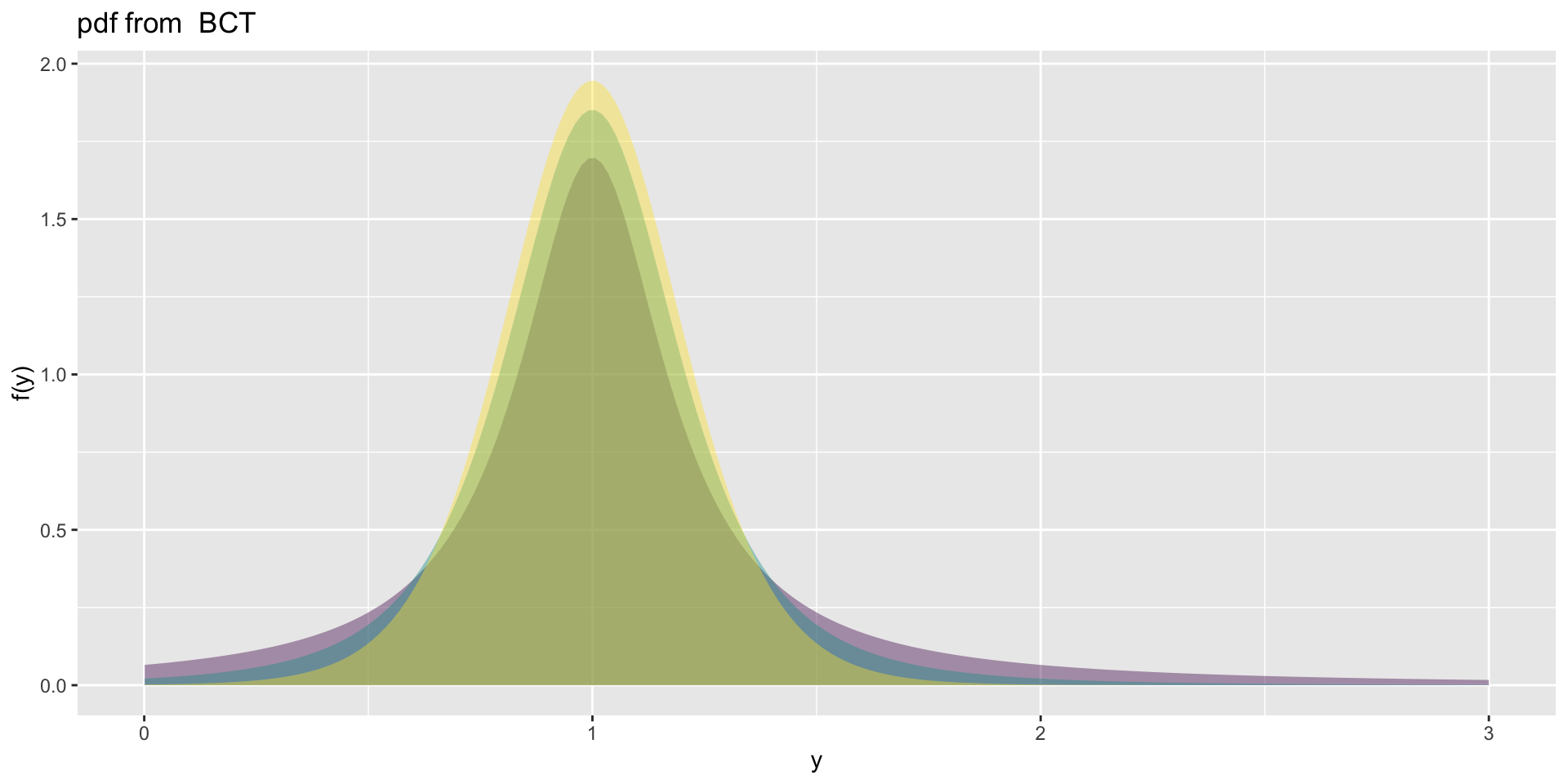
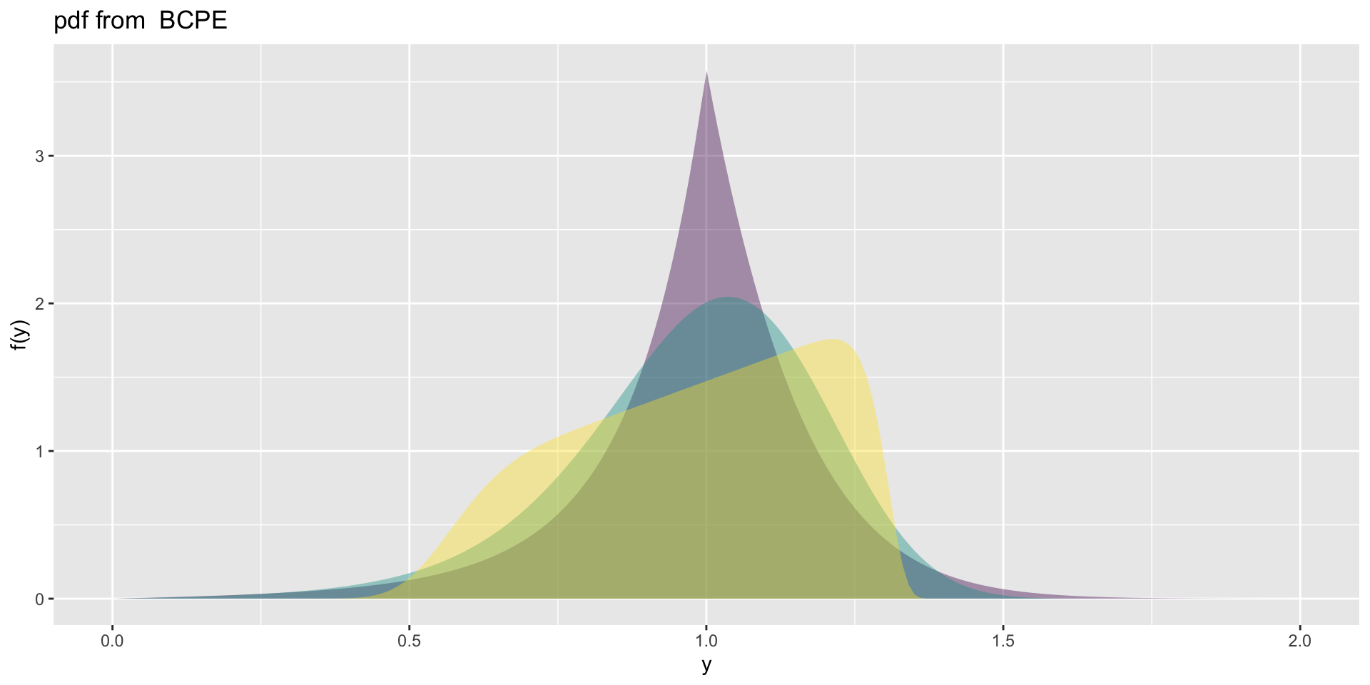
Box-Cox power exponential, \(\texttt{BCPE}(\mu,\sigma,\nu,\tau)\) and \(\texttt{BCPEo}(\mu,\sigma,\nu,\tau)\) skewness and platy-lepto;
Box-Cox t, \(\texttt{BCT}(\mu,\sigma,\nu,\tau)\) and \(\texttt{BCTo}(\mu,\sigma,\nu,\tau)\) skewness and leptokurtosis;
generalised beta type 2, \(\texttt{GB2}(\mu,\sigma,\nu,\tau)\) skewness and platy-lepto.

the BCT

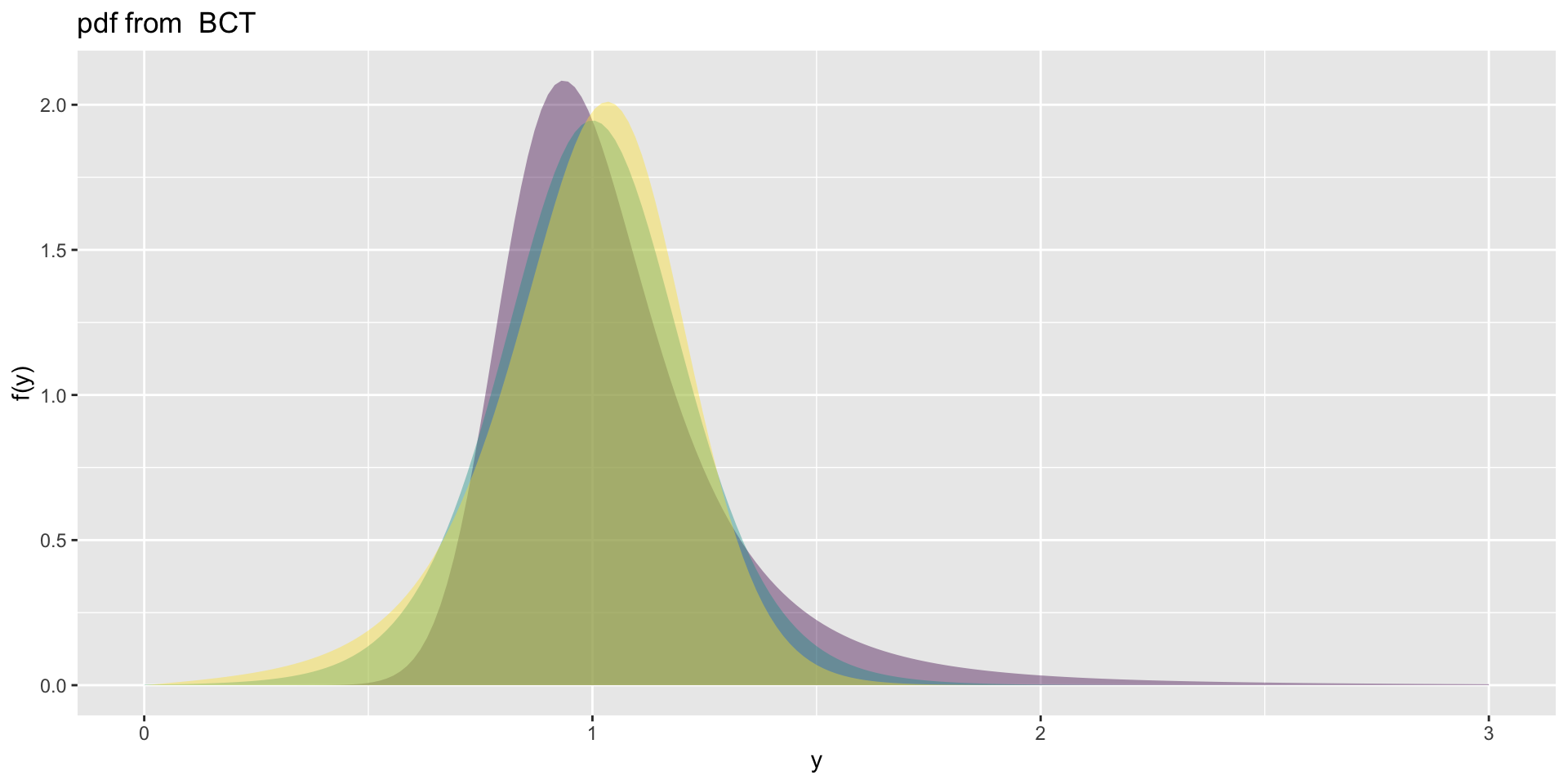
the BCT (con.)

the BCPE

Summary

Distributions	family	no par.	skewness	kurtosis
BCCG	`BCCG`	3	both
BCPE	`BCPE`	4	both	both
BCT	`BCT`	4	both	lepto
Exponential	`EXP`	1	(positive)	-
Gamma	`GA`	2	(positive)	-
Gen. Beta type 2	`GB2`	4	both	both
Gen. Gamma	`GG`-GG2	3	positive	-
Gen. Inv. Gaussian	`GIG`	3	positive	-
Inv. Gaussian	`IG`	2	(positive)	-
Log Normal	`LOGNO`	2	(positive)	-
Log Normal family	`LNO`	2,(1)	positive
Reverse Gen. Extreme	`RGE`	3	positive	-
Weibull	`WEI`, `WEI2`, `WEI3`	2	(positive)

{.striped .hover}

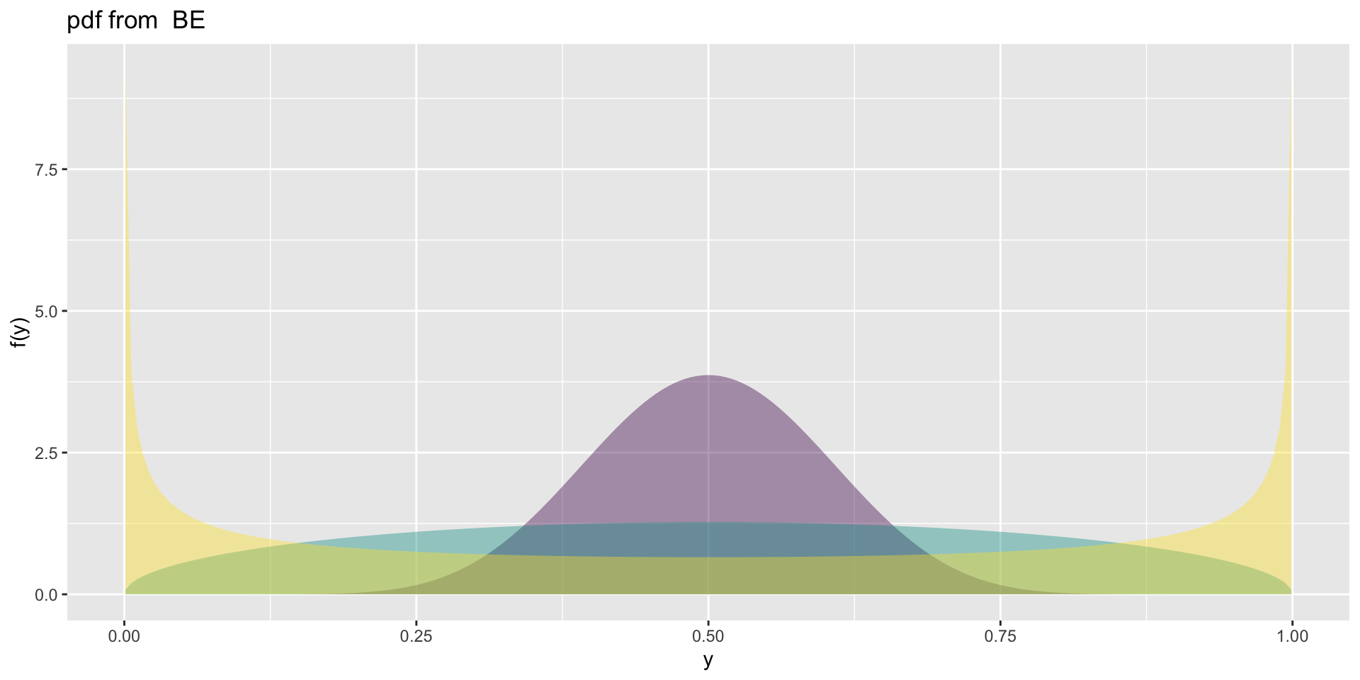
Explicit Distributions on \(\Re_{(0,1)}\)

Distributions on \(\Re_{(0,1)}\)

Distributions	family	no par.	skewness/kurtosis
beta	`BE`	2	(both)
beta original	`BEo`	2	(both)
generalized beta type 1	`GB1`	4	both
logit normal	`LOGITNO`	2	(both)
simplex	`SIMPEX`	2	(both)

the BE

Choosing distributions

Choosing distribution

global deviance

\[ \begin{split} GDEV=& -2\ell(\boldsymbol{\hat{\theta}}) =& -2 \sum_{i=1}^n \log f(y_i |\boldsymbol{\hat{\theta}}) \end{split}\]

generalized Akaike information criterion \[ GAIC(k) = GDEV + k \cdot df \] special cases \[\begin{split} {\rm AIC} &= \texttt{GDEV}+2 \, df\\ {\rm SBC} &= \texttt{GDEV}+ \log n \cdot df\ . \end{split}\]

Choosing distribution

prediction global deviance

\[\begin{split} TDEV=& -2, \ell (\boldsymbol{\widetilde{\theta}}) \\ =& -2\sum_{i=1}^{n_P} \log f( \widetilde{y}_i | \widetilde{\boldsymbol{\theta}}) \end{split}\]

\({\widetilde{ y}}\) indicates the response variable values at the validation (or test) sample,

How to fit distributions in R

optim() or mle() R functions requiring initial parameter values
gamlsssML() fits a distribution (using MLE) on the response with no explanatory variables
gamlss() fits a distribution on the response using RS or CG or mixed algorithms,
histDist() fits a distribution using gamlsssML(), and plots a histogram of the response with the fitted distribution
fitDist() fits a set of distributions to the response and chooses the one with the smallest GAIC
chooseDist() fits a set of distributions on a fitted model and chooses the one with the smallest GAIC

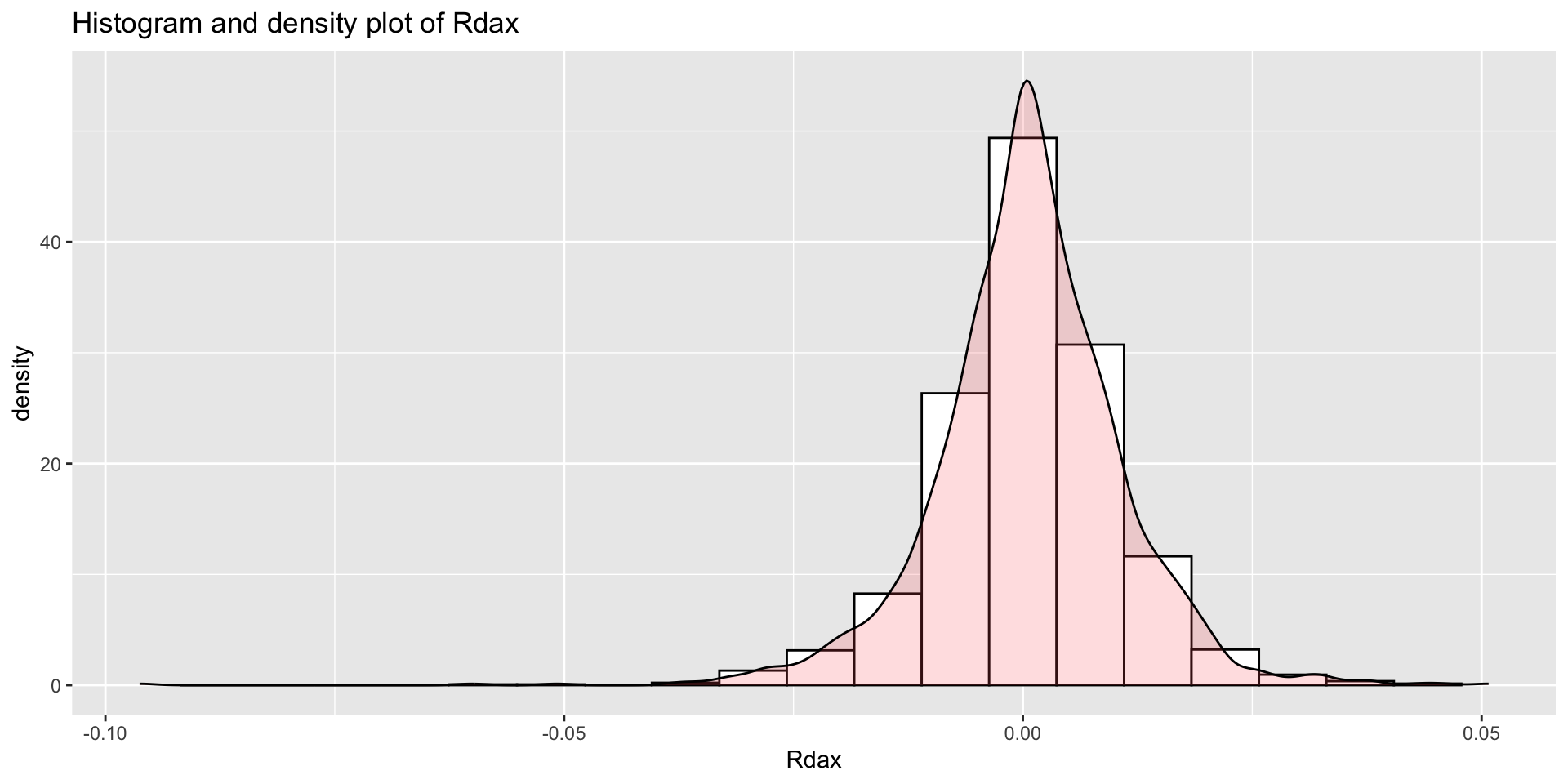
Example: DAX returns data

data(EuStockMarkets)
dax <-EuStockMarkets[,"DAX"]
Rdax <- diff(log(dax))
plot(Rdax)

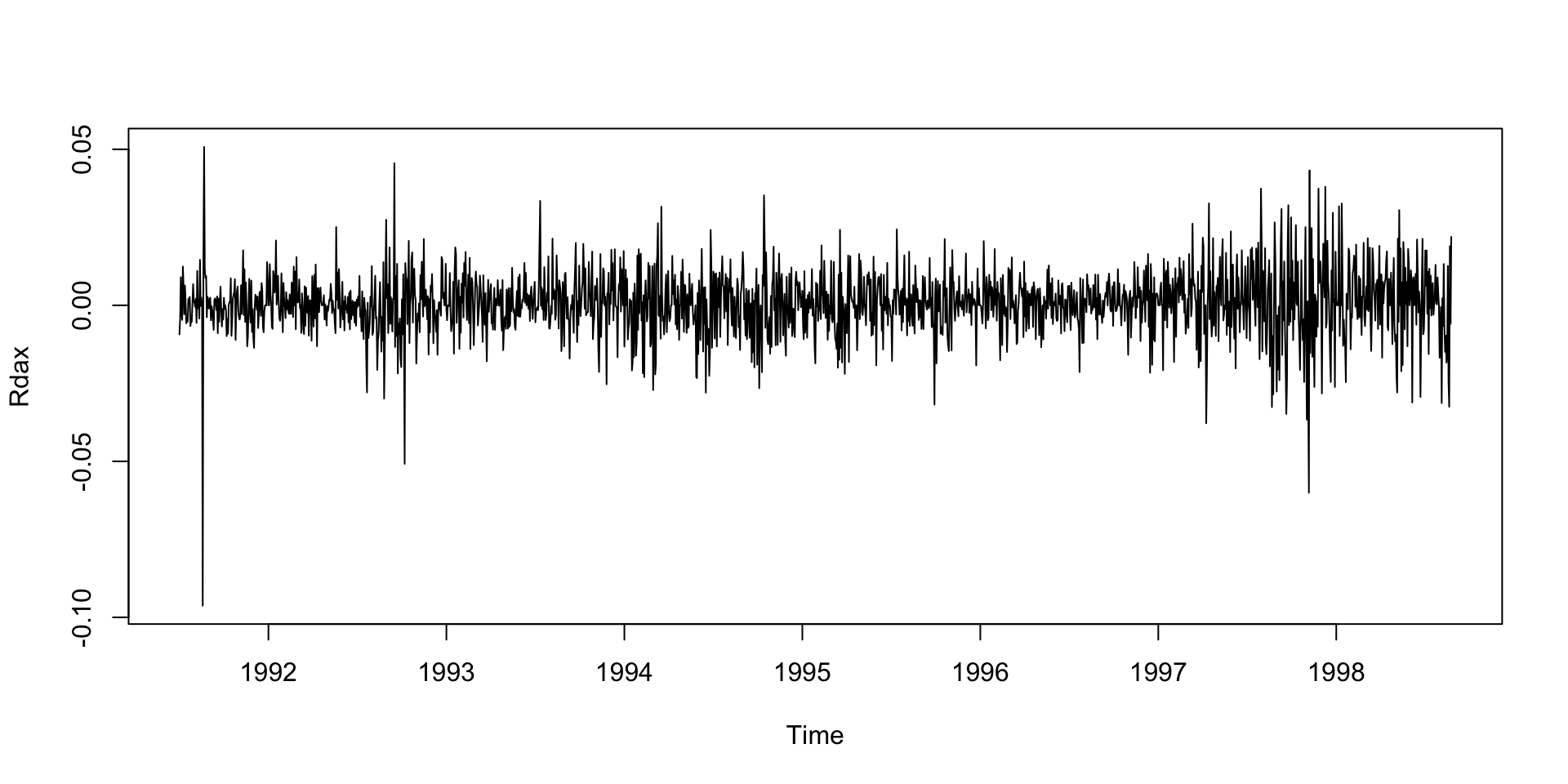
Example: DAX returns data (con.)

library(gamlss.ggplots)
y_hist(Rdax)

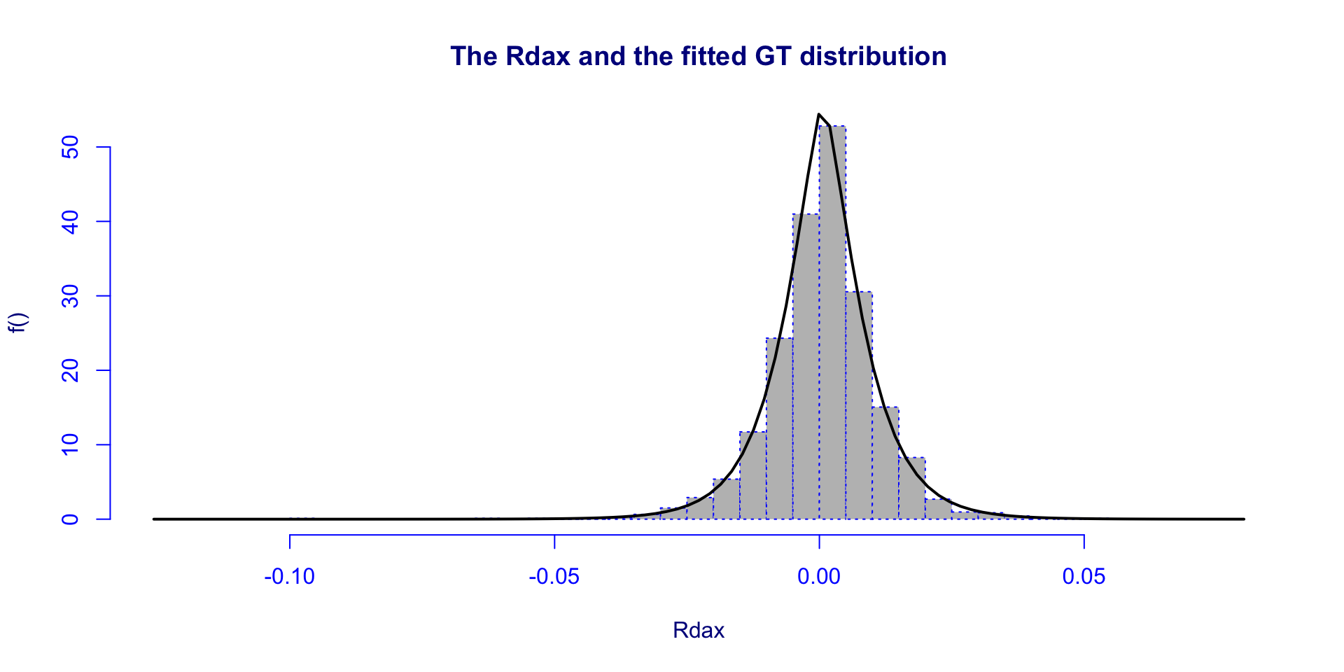
`fitDist()`

f1 <- fitDist(Rdax)

f1$fits

        GT       SEP2         PE        PE2        JSU       JSUo       SEP1 
-11967.683 -11965.533 -11962.464 -11962.464 -11961.477 -11961.477 -11961.305 
      SEP4       SEP3        TF2         TF        ST4        ST1       EGB2 
-11961.274 -11960.823 -11960.644 -11960.644 -11960.153 -11959.833 -11959.701 
       ST5        ST2        ST3        SST      SHASH    SHASHo2     SHASHo 
-11959.479 -11959.280 -11958.866 -11958.866 -11957.538 -11956.241 -11956.241 
        LO        NET        SN1        SN2         NO     exGAUS         GU 
-11932.112 -11919.175 -11759.871 -11739.127 -11733.208 -11733.171 -11262.120 
        RG         GA         GG        GB2       BCTo      BCCGo      BCPEo 
-10249.878  -7506.758  -7506.702  -7506.330  -7505.499  -7503.496  -7503.111 
       EXP    PARETO2   PARETO2o         IG     IGAMMA 
 -7481.488  -7479.488  -7479.487  -6705.703  -6486.337

`chooseDist()`

GAMLSS-RS iteration  1: Global Deviance = -11737.208 eps = 0.000000

minimum GAIC(k= 2 ) family: GT 
minimum GAIC(k= 3.84 ) family: GT 
minimum GAIC(k= 7.53 ) family: PE

GAIG with k= 2

       GT      SEP2        PE       PE2       JSU      SEP1 
-11966.32 -11965.46 -11962.46 -11962.21 -11961.45 -11961.16

`chooseDist()`(con.)

m2 <- gamlss2(Rdax~1, family=GT, trace=FALSE)
fitted(m2, parameter="mu", type="parameter")[1,1]

[1] 0.0007286232

fitted(m2, parameter="sigma", type="parameter")[1,2]

[1] 0.01005041

fitted(m2, parameter="nu", type="parameter")[1,3]

[1] 3.633405

fitted(m2, parameter="tau", type="parameter")[1,4]

[1] 1.603723

`histDist()`

m3 <- histDist(Rdax, family=GT, nbins=30, line.col="black")

practical 2

END

back to the index

The Books

Continuous Distributions

Types

Explicit distributions in real line, \(\Re\).

Location and Scale family

location

scale

2 parameter in \(\Re\)

2 parameter in \(\Re\) (con.)

2 parameter in \(\Re\) (con.)

3 parameter in \(\Re\)

3 parameter in \(\Re\) (con.)

3 parameter in \(\Re\) (con.)

3 parameter in \(\Re\) (TEST 1)

3 parameter in \(\Re\) PE

3 parameter in \(\Re\) PE (test)

3 parameter in \(\Re\) TF

3 parameter in \(\Re\) TF (test)

4 parameter in \(\Re\)

4 parameter in \(\Re\) (con.)

4 parameter in \(\Re\) SEP1

4 parameter in \(\Re\) SEP1

4 parameter in \(\Re\) SEP1

4 parameter in \(\Re\) SEP1

4 parameter in \(\Re\) NET

Summary

Explicit Distributions in positive real line \(\Re^+\)

the scale family

the weibull 3

the weibull 3 (con.)

1 and 2 parameter positive real line, \(\Re^+\).

Weibull survival and hazard

3 parameter positive real line \(\Re^+\)

the BCCG

the BCCG (con.)

4 parameter positive real line \(\Re^+\)

the BCT

the BCT (con.)

the BCPE

Summary

Explicit Distributions on \(\Re_{(0,1)}\)

Distributions on \(\Re_{(0,1)}\)

the BE

Choosing distributions

Choosing distribution

Choosing distribution

How to fit distributions in R

Example: DAX returns data

Example: DAX returns data (con.)

fitDist()

chooseDist()

chooseDist()(con.)

histDist()

practical 2

END

`Location` and `Scale` family

`fitDist()`

`chooseDist()`

`chooseDist()`(con.)

`histDist()`