Centile estimation
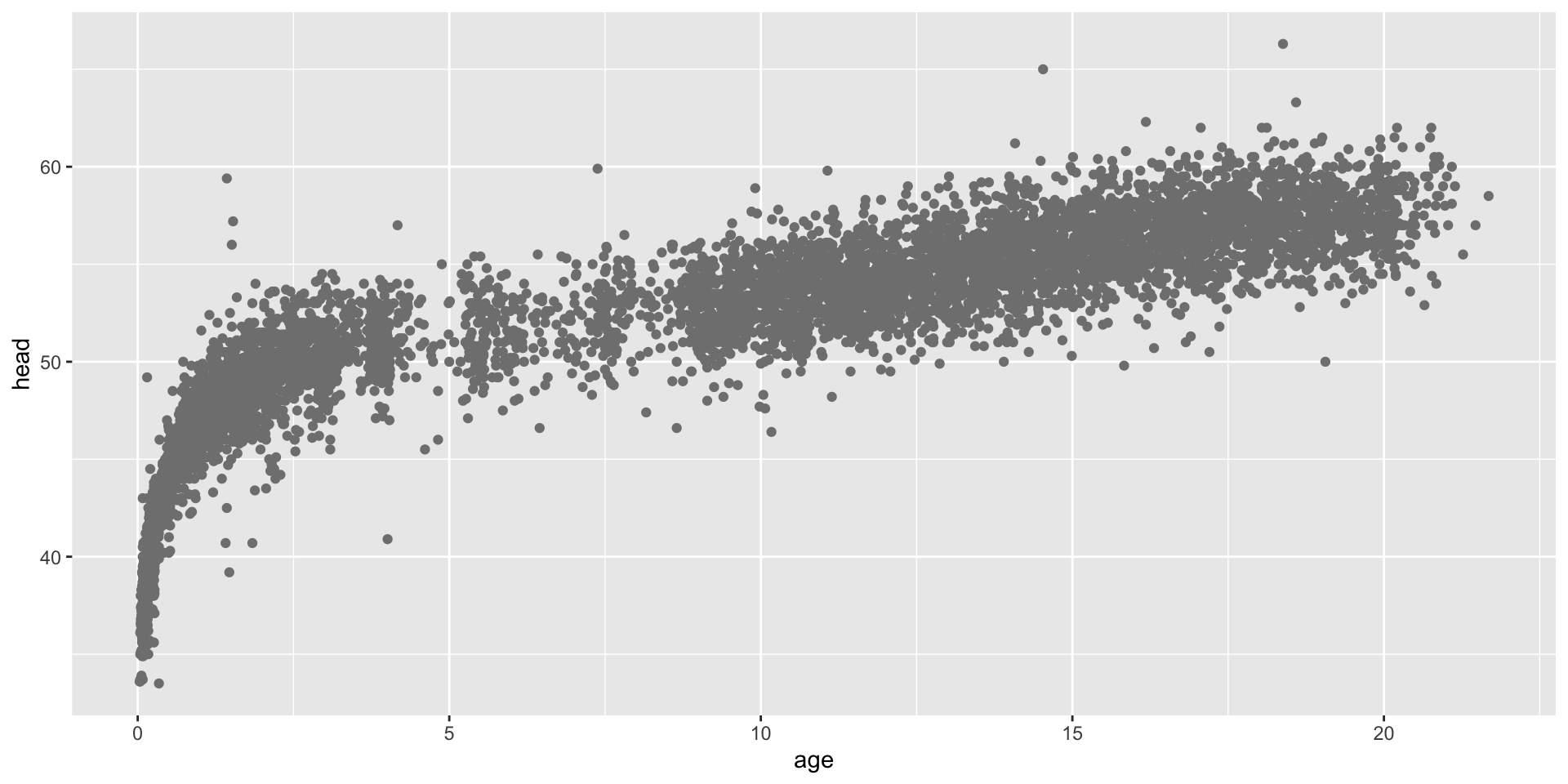
the data plot
estimate the curves

the target
Box-Cox & Cole-Green transformation
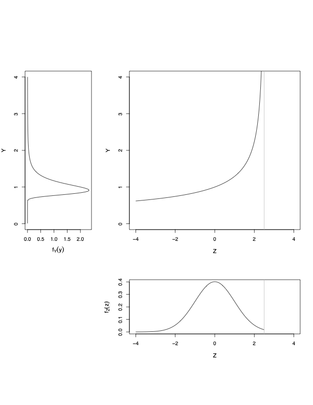
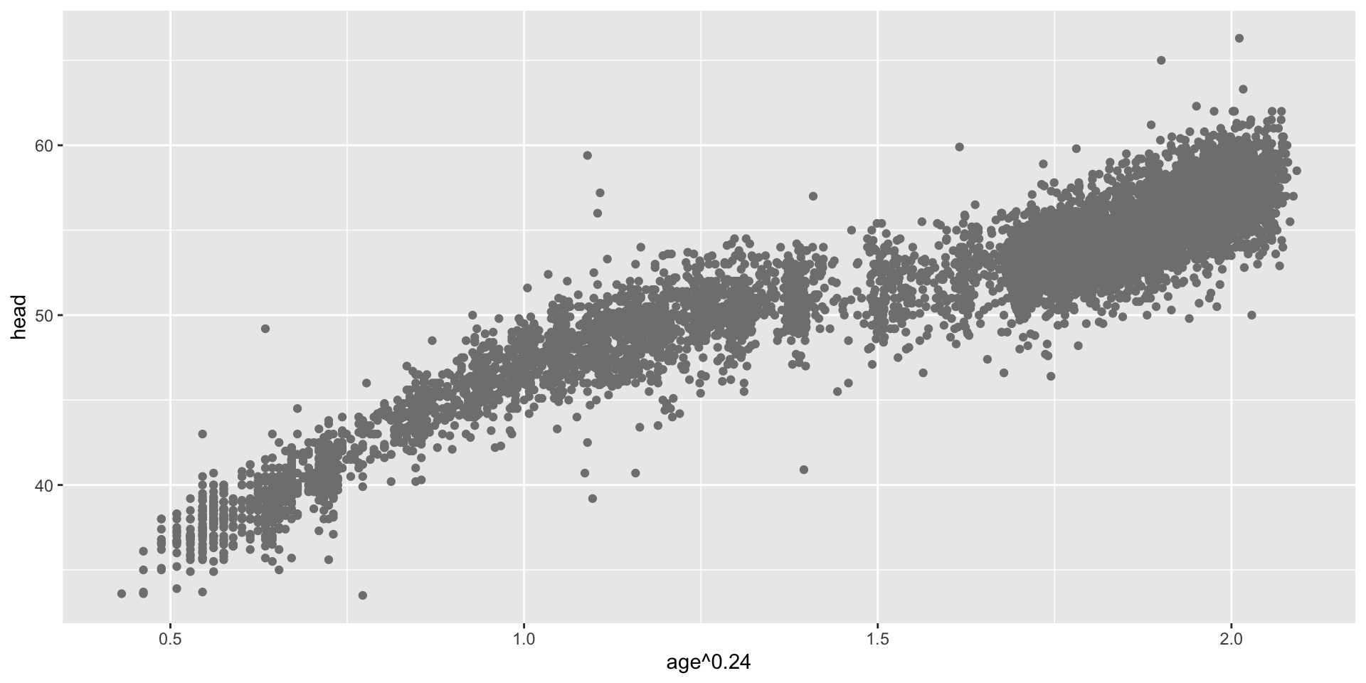
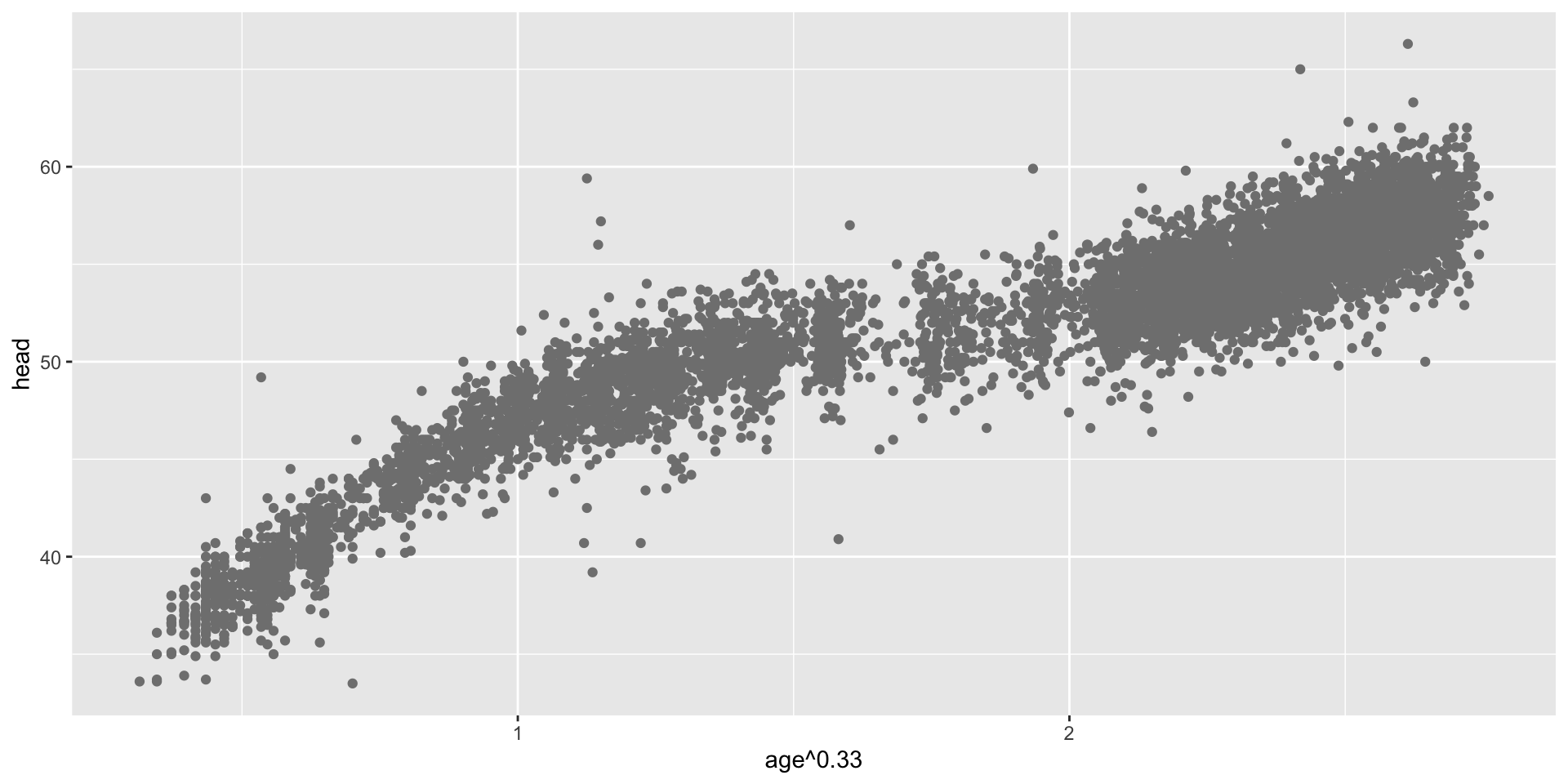
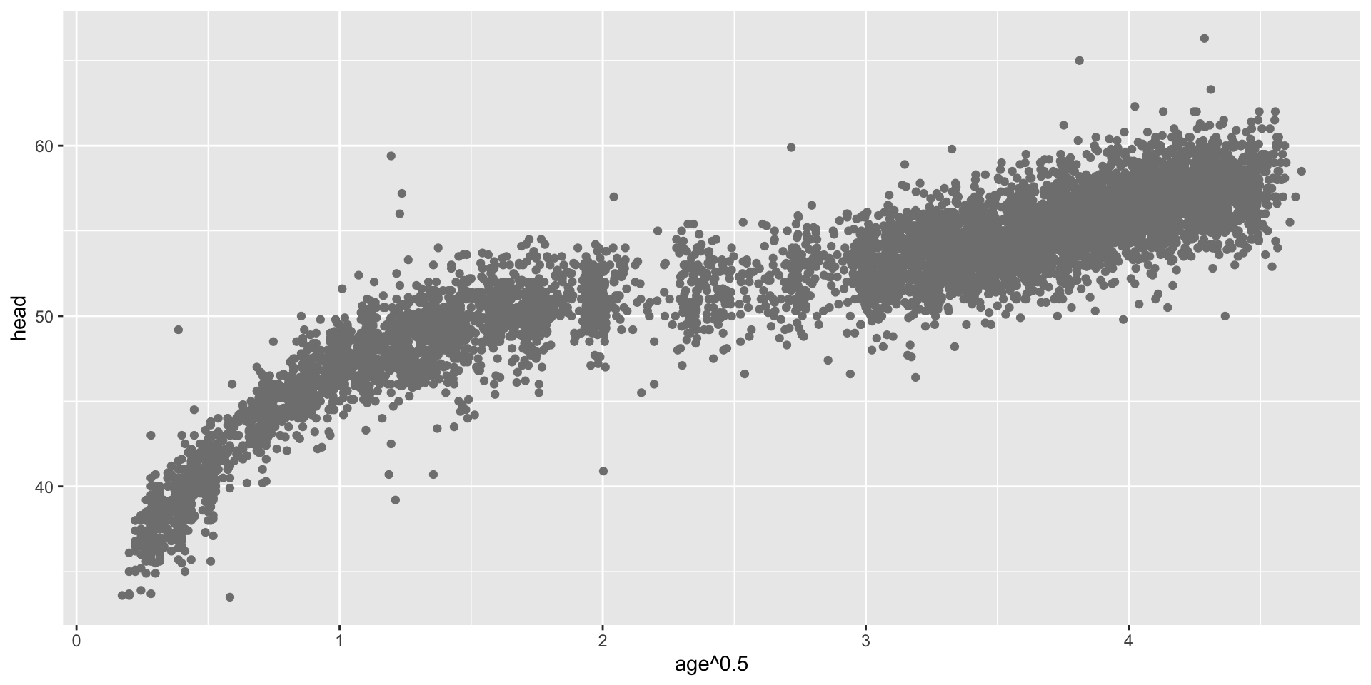
transformation parameter \(\xi\)
library(gamlss2)
library(gamlss.ggplots)
gamlss.ggplots:::find_power(y=db$head, x=db$age, profile=TRUE, from=0, to=1, step=0.01)
*** Checking for transformation for x *** *** power parameters 0.24 *** [1] 0.24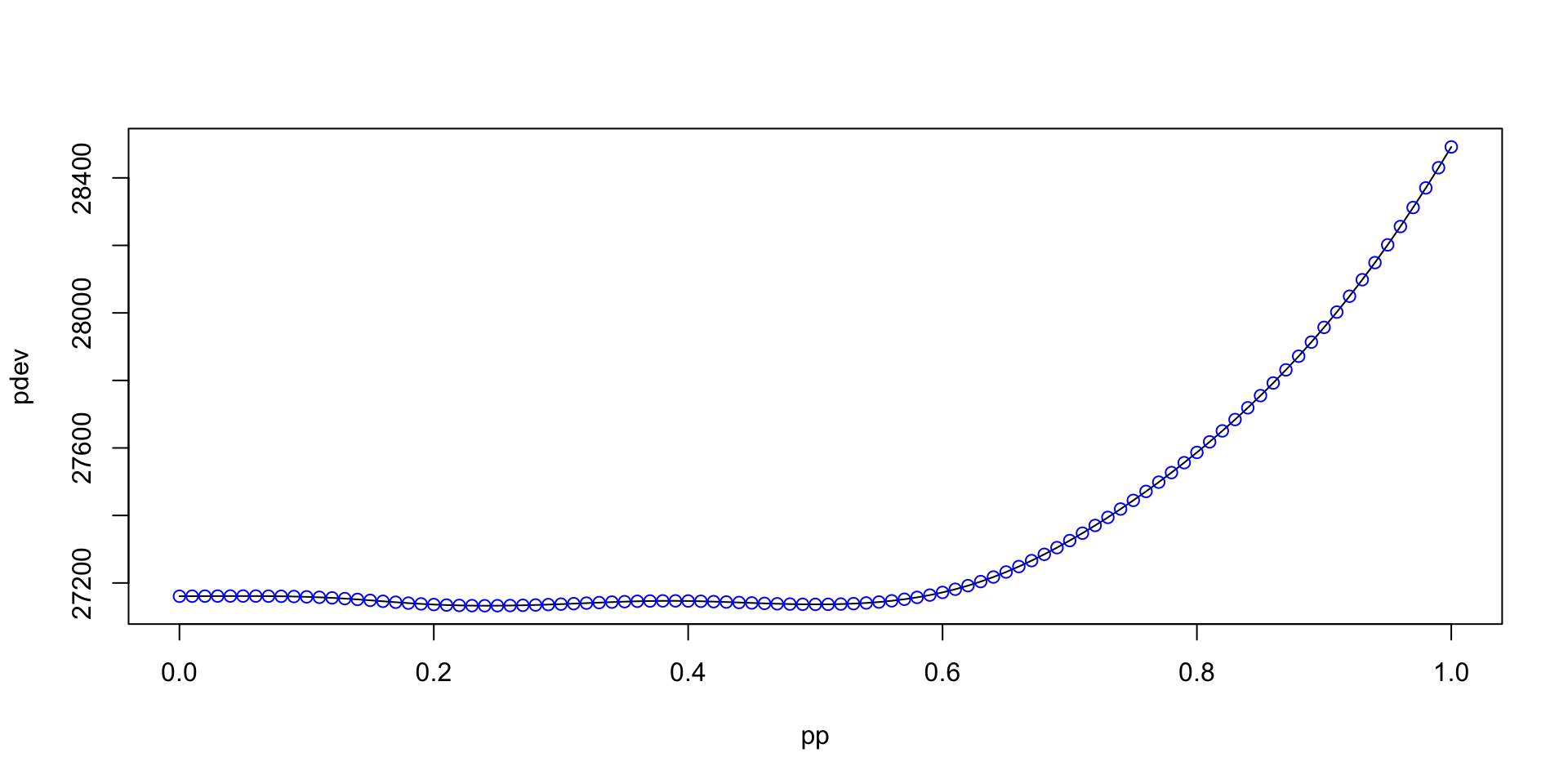
transformation parameter \(\xi\) (con.)
transformation parameter \(\xi\) (con.)
transformation parameter \(\xi\) (con.)
select models
            AIC       df
gBCTo  26792.07 22.08936
gBCPEo 26871.06 24.53565
gBCCGo 26998.12 28.14446
gNO    27042.92 18.91385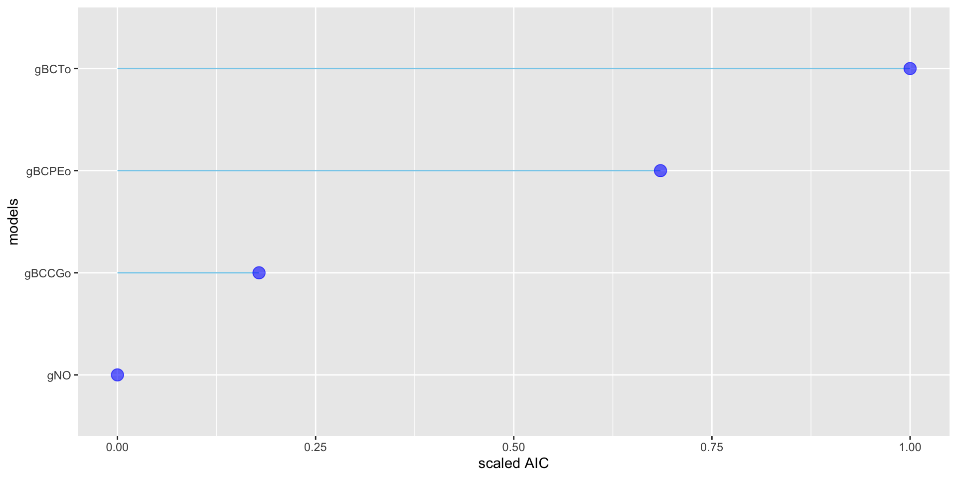
diagnostic tools: residuals
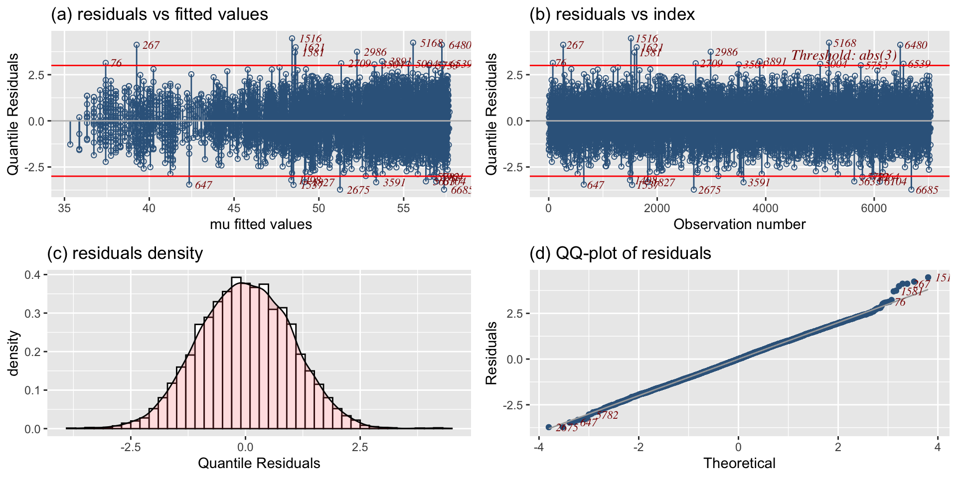
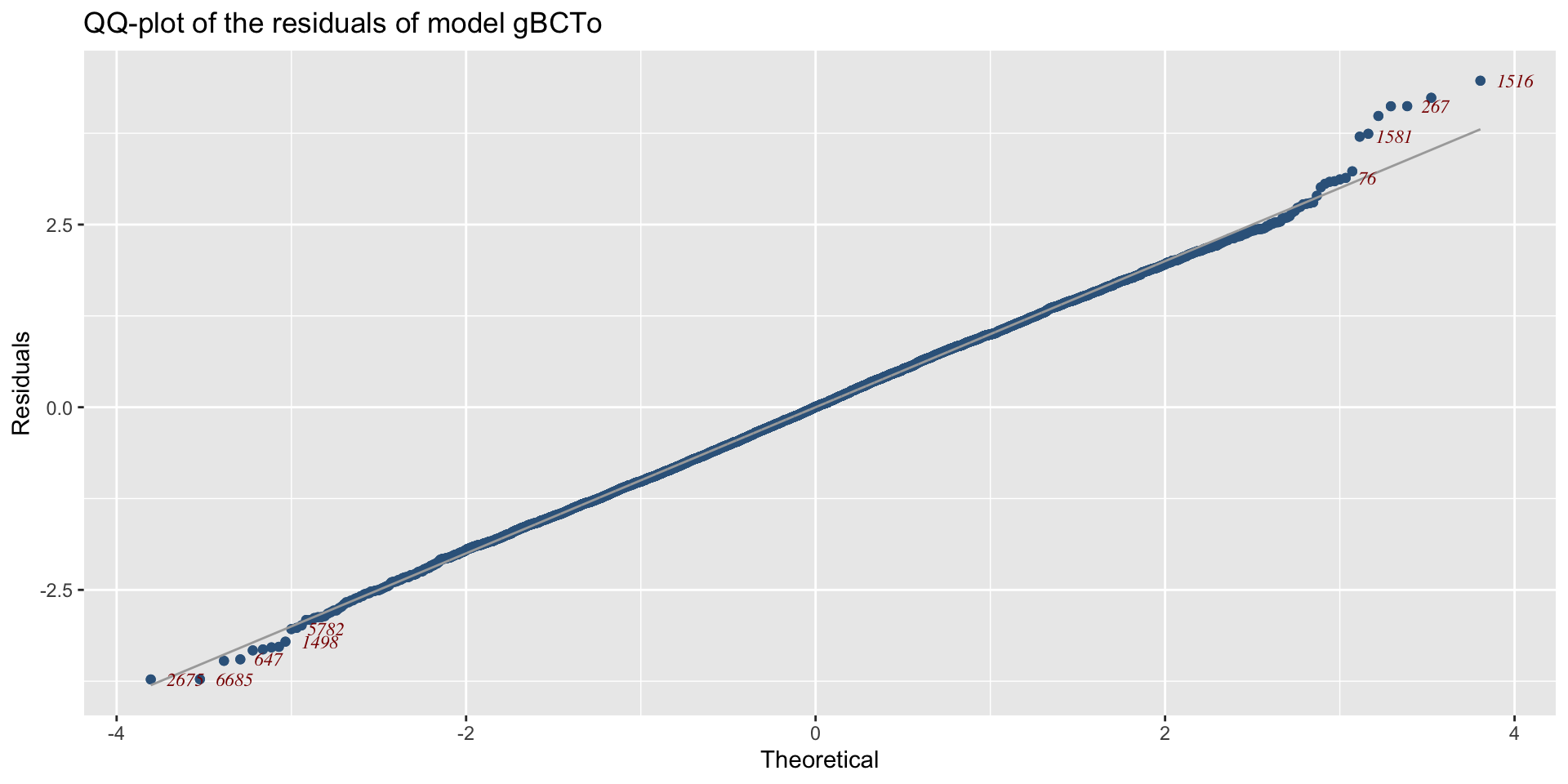
QQplot
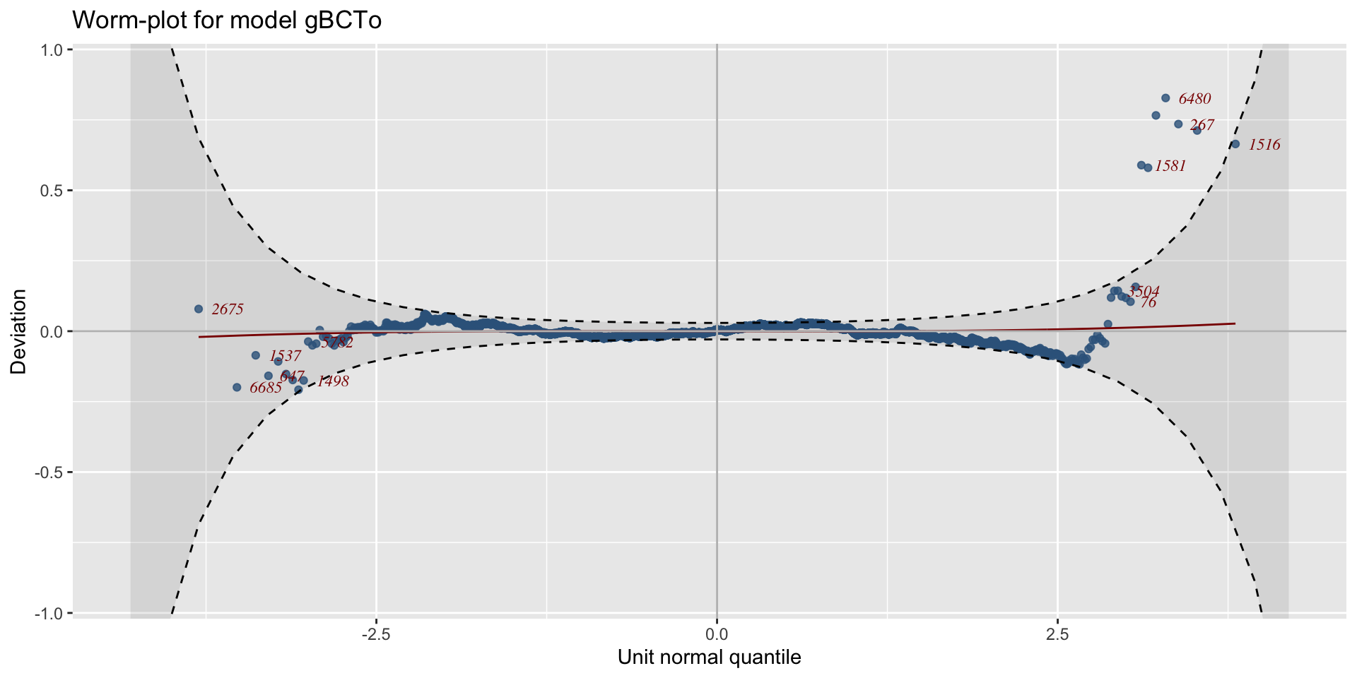
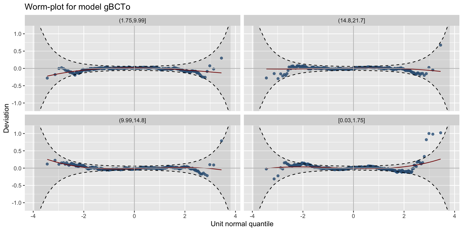
worm plots
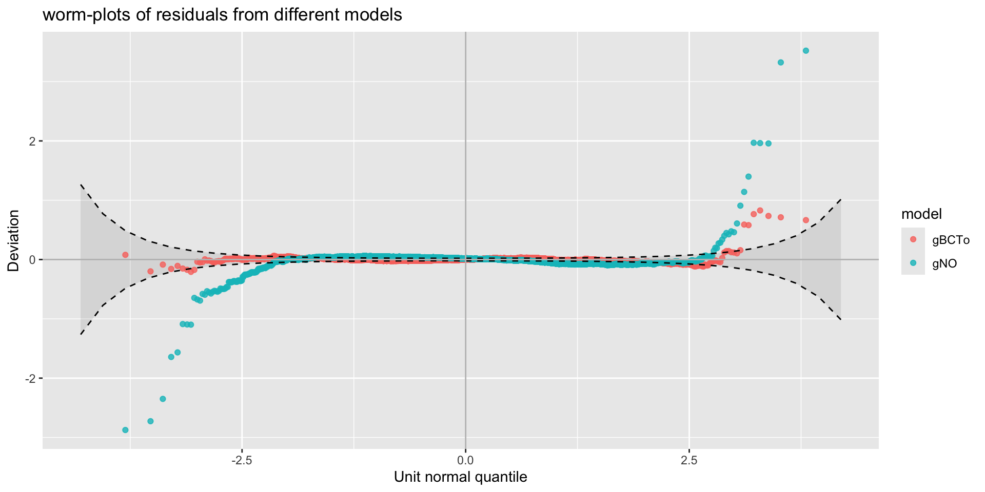
different models worm plots
different x-values worm plots
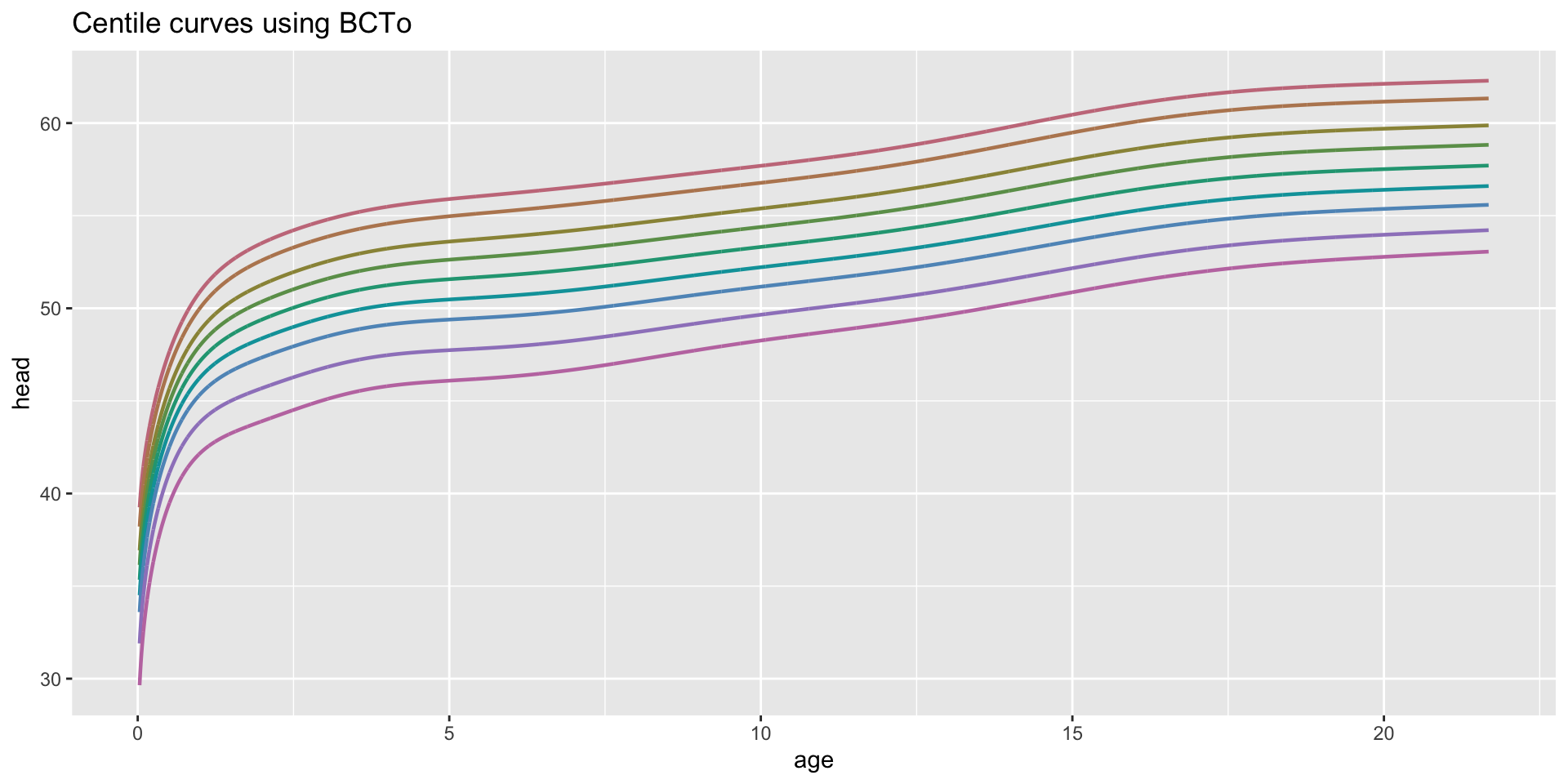
centiles
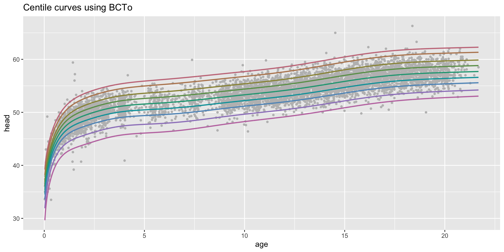
centiles just curves

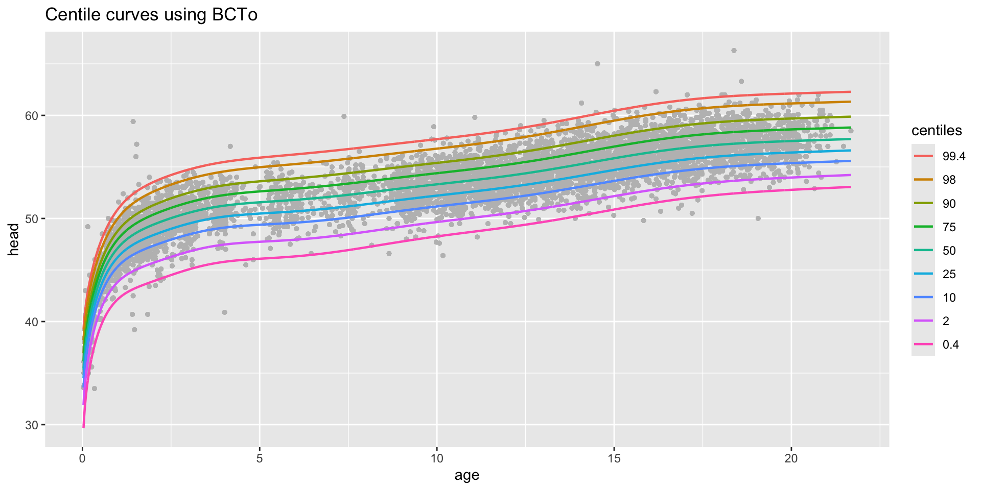
centiles with legend
centiles different models
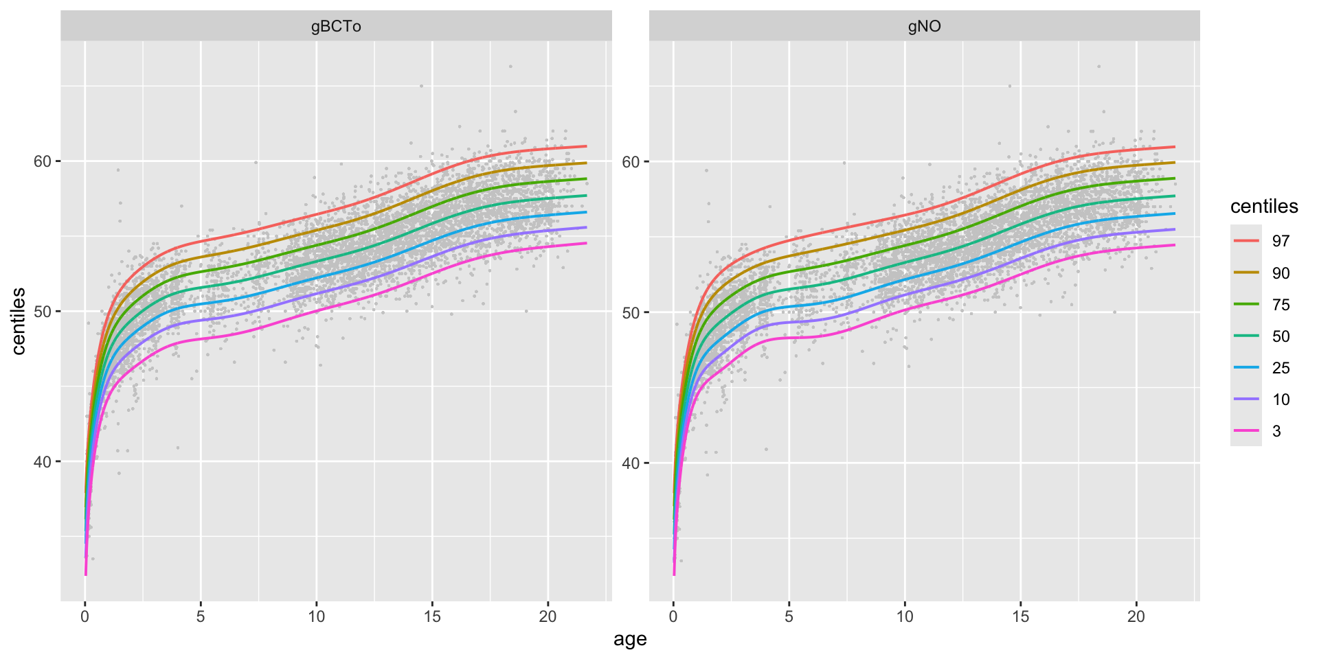
centiles different models in one plot
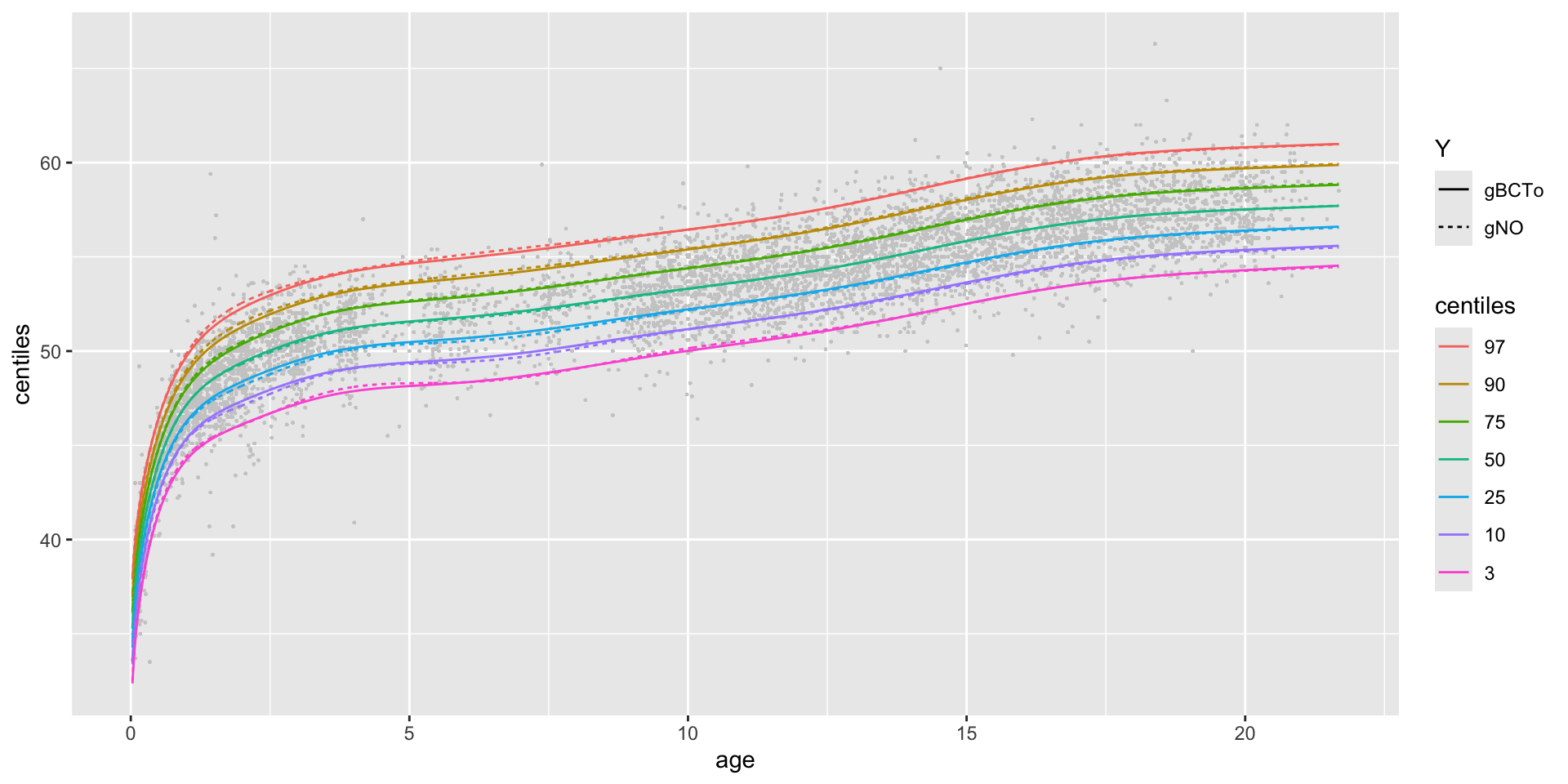
centiles different models in one plot

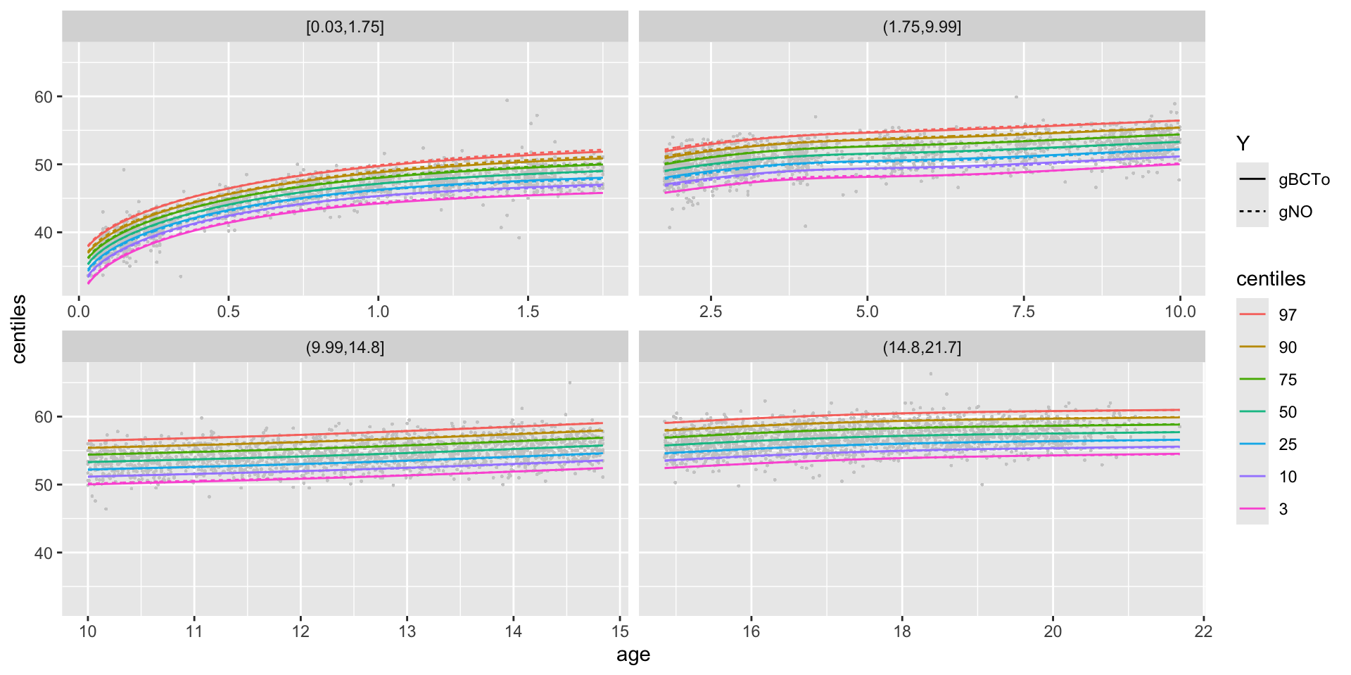
centiles different models different x-valus in one plot
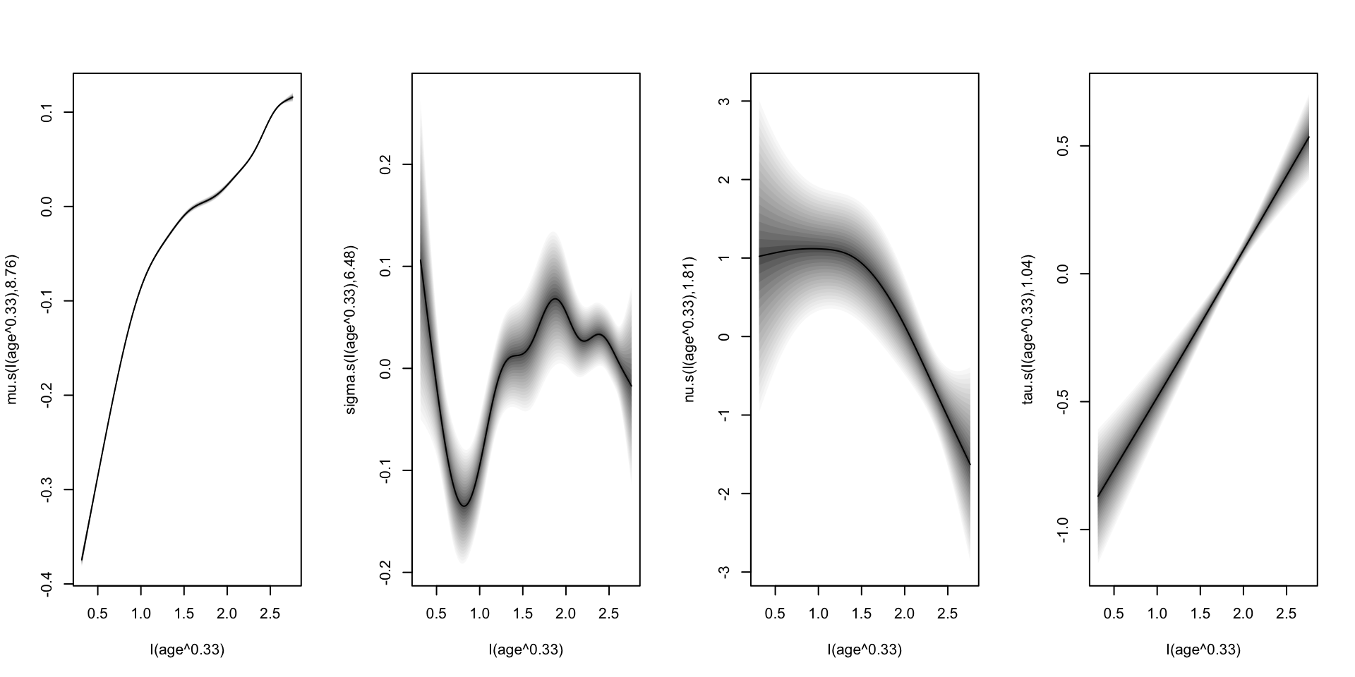
fitted parameters
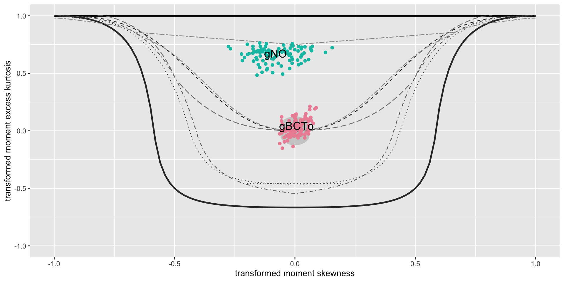
bucket plots
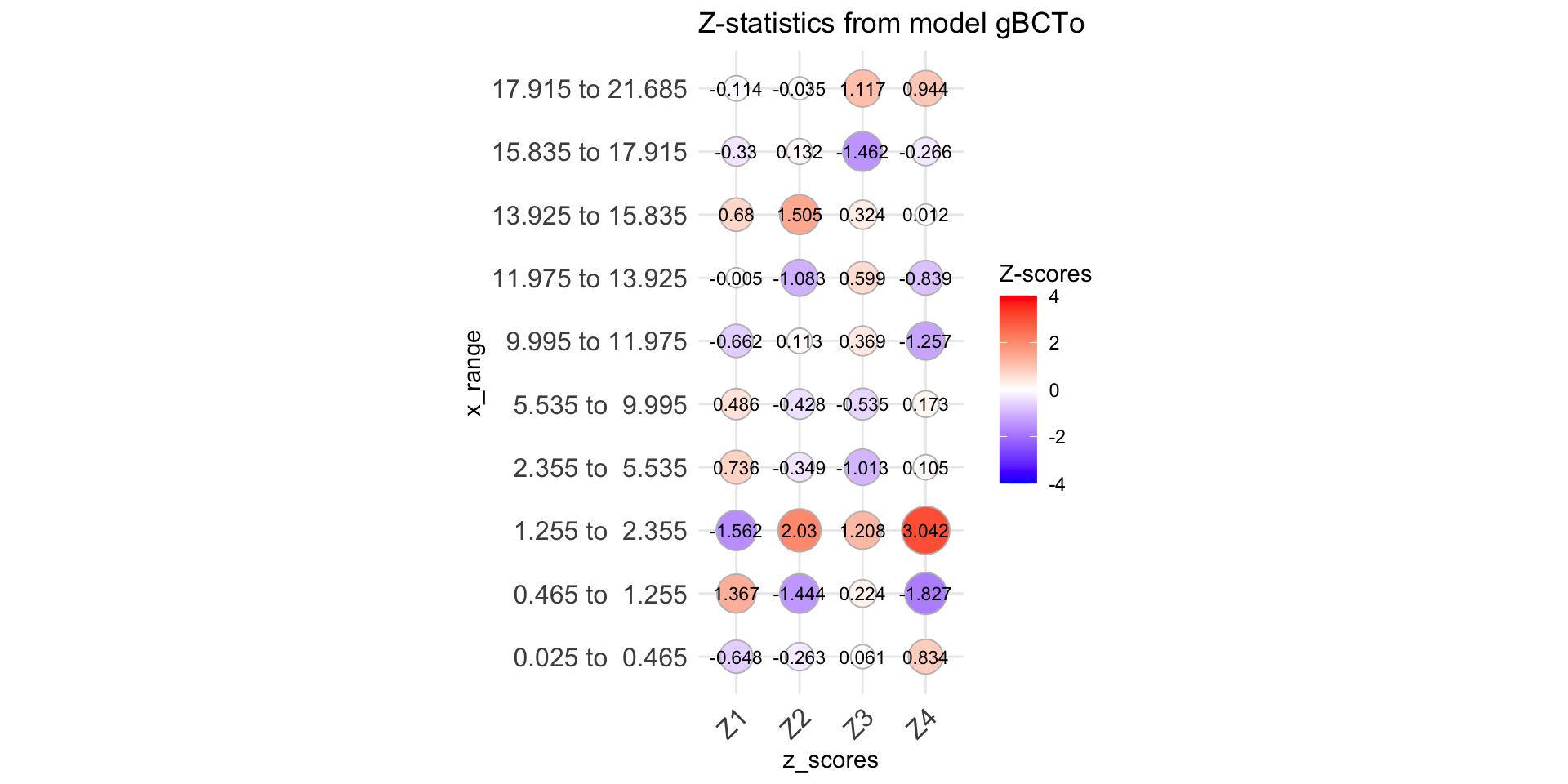
Q-stats
end
 The Books
![]()