Fitting models

Mikis Stasinopoulos

Bob Rigby

Fernanda De Bastiani

Gillian Heller

Niki Umlauf

Introduction

questions

• do my data support a GAMLSS model?

• do I need GAMLSS to answer my questions?

• size of the data

• questions of interest

this talk

• the basic GAMLSS algorithm
• different statistical approaches for fitting a GAMLSS model
• different machine learning techniques for fitting a GAMLSS model.

Algorithms

GAMLSS

\[\begin{split} y_i & \stackrel{\small{ind}}{\sim }& {D}( \theta_{1i}, \ldots, \theta_{ki}) \nonumber \\ g(\theta_{1i}) &=& b_{10} + s_1({x}_{1i}) + \ldots, s_p({x}_{pi}) \nonumber\\ \ldots &=& \ldots \nonumber\\ g({\theta}_{ki}) &=& b_0 + s_1({x}_{1i}) + \ldots, s_p({x}_{pi}) \end{split} \qquad(1)\]

for \(i=1,2,\ldots,n\).

GAMLSS + ML

\[\begin{split} y_i & \stackrel{\small{ind}}{\sim }& {D}( \theta_{1i}, \ldots, \theta_{ki}) \nonumber \\ g({\theta}_{1i}) &=& {ML}_1({x}_{1i},{x}_{2i}, \ldots, {x}_{pi}) \nonumber \\ \ldots &=& \ldots \nonumber\\ g({\theta}_{ki}) &=& {ML}_1({x}_{1i},{x}_{2i}, \ldots, {x}_{pi}) \end{split} \qquad(2)\]

two major problems

• The task within GAMLSS is to find ;

  1. how the x’s effect the parameters of the distribution i.e \(\boldsymbol{\theta}(X)\) and

  2. the appropriate distribution for the response i.e. \(D(Y|\boldsymbol{\theta}(X))\)

DISTRIBUTION

• The range of the response should determine the type of distribution

• if we know the right variables we could determine a adequate distribution by looking over a set of appropriate distributions

• if one of the variable is very important i.e. time, age it can be used otherwise use a linear model for all parameters (which works fast) to pick up a distribution

Parameters for Estimation

Given a distribution we need to estimate the;

• distribution parameters

• coefficient parameters

    - **coefficients**
  
    - **random effects** and the 

• hyper-parameters

flowchart

flowchart LR
  A[GAMLSS] --> L[Parametric]
  A --> N[Smooth]
  L --> B(Likelihood)
  L --> D(Bayesian)
  L --> E(Boosting)
  N --> C(Penalised Likelihood)
  N --> D(Bayesian)
  N --> E(Boosting)
  B --> G[beta's]
  C --> F[beta's, gamma's, & lambda's]
  E --> F
  D --> F
  D --> G
  E --> G

Figure 1: Different ways to estimate the parameters in a GAMLSS model.

The Basic Algorithm for GAMLSS

• For specified distribution family, data and machine learning (ML) model.

Initialize: set starting values for all distribution parameters \((\hat{\boldsymbol{\mu}}^{(0)}, \hat{\boldsymbol{\sigma}}^{(0)}, \hat{\boldsymbol{\nu}}^{(0)}, \hat{\boldsymbol{\tau}}^{(0)} )\).

For i in \(1,2,\ldots\)

• fix \(\hat{\boldsymbol{\sigma}}^{(i-1)}\),\(\hat{\boldsymbol{\nu}}^{(i-1)}\), and \(\hat{\boldsymbol{\tau}}^{(i-1)}\) and fit a ML model to iterative response \(\textbf{y}_{\mu}\) using iterative weights \(\textbf{w}_{\mu}\) to obtain the new \(\hat{\boldsymbol{\mu}}^{(i)}\)

• fix \(\hat{\boldsymbol{\mu}}^{(i)}\),\(\hat{\boldsymbol{\nu}}^{(i-1)}\), and \(\hat{\boldsymbol{\tau}}^{(i-1)}\) and fit a ML model to iterative response \(\textbf{y}_{\sigma}\) using iterative weights \(\textbf{w}_{\sigma}\) to obtain the new \(\hat{\boldsymbol{\sigma}}^{(i)}\)

• fix \(\hat{\boldsymbol{\mu}}^{(i)}\),\(\hat{\boldsymbol{\sigma}}^{(i)}\), and \(\hat{\boldsymbol{\tau}}^{(i-1)}\) and fit a ML model to iterative response \(\textbf{y}_{\nu}\) using iterative weights \(\textbf{w}_{\nu}\) to obtain the new \(\hat{\boldsymbol{\nu}}^{(i)}\)

• fix \(\hat{\boldsymbol{\mu}}^{(i)}\),\(\hat{\boldsymbol{\sigma}}^{(i)}\), and \(\hat{\boldsymbol{\nu}}^{(i)}\) and fit a ML model to iterative response \(\textbf{y}_{\tau}\) using iterative weights \(\textbf{w}_{\tau}\) to obtain the new \(\hat{\boldsymbol{\nu}}^{(i)}\)

• check if the global deviance, \(-2(\textit{log-likelihood})\) does not change repeat otherwise exit

Important

• for the assumed distribution the log-likelihood is needed (and the first and second derivatives with respect to the parameters)

• an hierarchy of the parameters exist a good location model is required before model the scale parameters e.t.c.

• orthogonality of the parameters leads to better convergence and interpretation

Checking orthogonality

• Specify a distribution family, and select values for all the parameters.

• generate a sample of of N observations (default \(N=10000\))

• fit the distribution to the generated sample.

• display the correlation coefficients of the estimated predictors, \(\eta_{\theta}\).

Checking orthogonality (con.)

source("~/Dropbox/GAMLSS-development/ggplot/family_cor.R")
library(gamlss)
library(ggplot2)
family_cor("BCTo", mu=1, sigma=0.11, nu=1, tau=5, no.sim=10000)

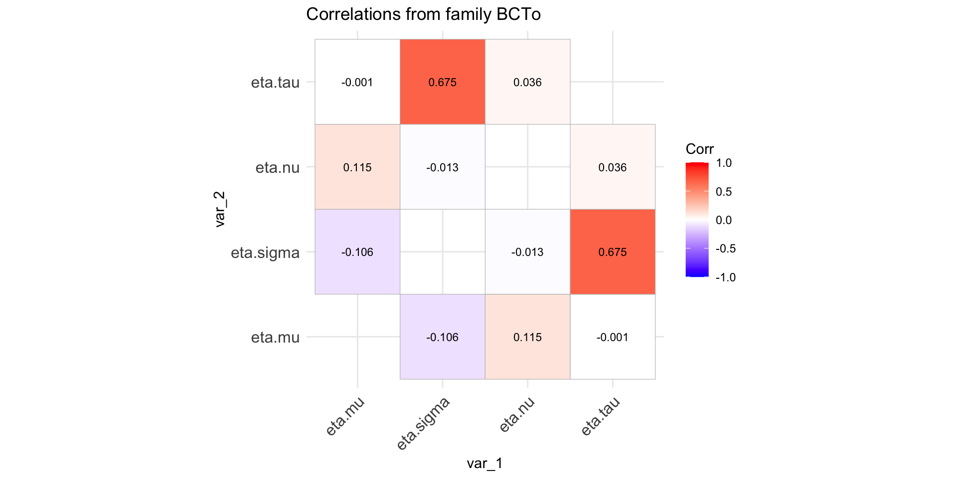
Figure 2: Paramater orthogonality for BCTo distribution

Machine Learning Models

properties

• are the standard errors available?

• do the x’s need standardization.

• about the algorithm

   - stability
   - speed 
   - convergence    

• nonlinear terms

• interactions

• dataset type

• is the selection of x’s automatic?

• interpretation

Linear Models

mlinear <- gamlss2(rent~poly(area,3)+poly(yearc,3)+location+bath+kitchen+
              cheating|poly(area,3)+poly(yearc,3)+location+bath+kitchen+cheating, 
              family=BCTo, trace=FALSE, data=da)
summary(mlinear)

Linear Models

Call:
gamlss2(formula = rent ~ poly(area, 3) + poly(yearc, 3) + location + 
    bath + kitchen + cheating | poly(area, 3) + poly(yearc, 3) + 
    location + bath + kitchen + cheating, data = da, family = BCTo, 
    ... = pairlist(trace = FALSE))
---
Family: BCTo 
Link functions: mu = log, sigma = log, nu = identity, tau = log
*--------
Coefficients:
                      Estimate Std. Error t value Pr(>|t|)    
mu.(Intercept)         5.71590    0.02366 241.595  < 2e-16 ***
mu.location2           0.09005    0.01028   8.760  < 2e-16 ***
mu.location3           0.21550    0.03717   5.798 7.39e-09 ***
mu.bath1               0.05882    0.02083   2.824  0.00478 ** 
mu.kitchen1            0.11118    0.02360   4.710 2.58e-06 ***
mu.cheating1           0.34265    0.02422  14.148  < 2e-16 ***
mu.poly(area, 3)1     13.33793    0.31111  42.871  < 2e-16 ***
mu.poly(area, 3)2     -2.01312    0.32273  -6.238 5.05e-10 ***
mu.poly(area, 3)3      0.63310    0.30519   2.074  0.03812 *  
mu.poly(yearc, 3)1     4.77815    0.34420  13.882  < 2e-16 ***
mu.poly(yearc, 3)2     3.66120    0.28934  12.654  < 2e-16 ***
mu.poly(yearc, 3)3    -0.76633    0.29134  -2.630  0.00857 ** 
sigma.(Intercept)     -1.16028    0.05323 -21.799  < 2e-16 ***
sigma.location2        0.05851    0.02972   1.969  0.04905 *  
sigma.location3        0.21471    0.09343   2.298  0.02162 *  
sigma.bath1            0.03078    0.06067   0.507  0.61191    
sigma.kitchen1         0.01141    0.07309   0.156  0.87597    
sigma.cheating1       -0.23024    0.05114  -4.502 6.98e-06 ***
sigma.poly(area, 3)1   1.90318    0.84748   2.246  0.02479 *  
sigma.poly(area, 3)2  -0.70530    0.81681  -0.863  0.38794    
sigma.poly(area, 3)3   1.23728    0.83095   1.489  0.13659    
sigma.poly(yearc, 3)1 -7.40430    0.89183  -8.302  < 2e-16 ***
sigma.poly(yearc, 3)2 -0.42953    0.81051  -0.530  0.59619    
sigma.poly(yearc, 3)3  3.66610    0.78688   4.659 3.31e-06 ***
nu.(Intercept)         0.68241    0.05732  11.906  < 2e-16 ***
tau.(Intercept)        3.12679    0.36811   8.494  < 2e-16 ***
---
Signif. codes:  0 '***' 0.001 '**' 0.01 '*' 0.05 '.' 0.1 ' ' 1
*--------
n = 3082 df =  26 res.df =  3056
Deviance = 38164.1012 Null Dev. Red. = 6.18%
AIC = 38216.1012 elapsed =  0.50sec

Additive Models

madditive <- gamlss2(rent~s(area)+s(yearc)+location+bath+kitchen+
                cheating|s(area)+s(yearc)+location+bath+kitchen+cheating, 
              family=BCTo, data=da, trace=F)
GAIC(mlinear, madditive)

               AIC       df
madditive 38196.79 31.99106
mlinear   38216.10 26.00000

GAIC(mlinear, madditive, k=log(dim(rent99)[1]))

               AIC       df
mlinear   38372.97 26.00000
madditive 38389.81 31.99106

Additive Models (con.)

summary(madditive)

Call:
gamlss2(formula = rent ~ s(area) + s(yearc) + location + bath + 
    kitchen + cheating | s(area) + s(yearc) + location + bath + 
    kitchen + cheating, data = da, family = BCTo, ... = pairlist(trace = F))
---
Family: BCTo 
Link functions: mu = log, sigma = log, nu = identity, tau = log
*--------
Coefficients:
                  Estimate Std. Error t value Pr(>|t|)    
mu.(Intercept)     5.71441    0.02085 274.133  < 2e-16 ***
mu.location2       0.08788    0.01102   7.977 2.11e-15 ***
mu.location3       0.20994    0.04962   4.231 2.39e-05 ***
mu.bath1           0.05822    0.04262   1.366  0.17206    
mu.kitchen1        0.10870    0.03636   2.990  0.00281 ** 
mu.cheating1       0.34716    0.02024  17.148  < 2e-16 ***
sigma.(Intercept) -1.15391    0.03702 -31.168  < 2e-16 ***
sigma.location2    0.05338    0.02264   2.358  0.01845 *  
sigma.location3    0.21232    0.08615   2.464  0.01378 *  
sigma.bath1        0.03452    0.08290   0.416  0.67713    
sigma.kitchen1     0.01909    0.07583   0.252  0.80122    
sigma.cheating1   -0.23645    0.03761  -6.288 3.69e-10 ***
nu.(Intercept)     0.69396    0.04544  15.272  < 2e-16 ***
tau.(Intercept)    3.27139    0.07556  43.292  < 2e-16 ***
---
Signif. codes:  0 '***' 0.001 '**' 0.01 '*' 0.05 '.' 0.1 ' ' 1
---
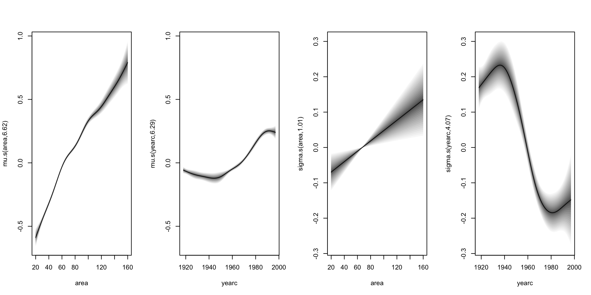
Smooth terms:
    mu.s(area) mu.s(yearc) sigma.s(area) sigma.s(yearc)
edf     6.6206      6.2852        1.0123         4.0731
*--------
n = 3082 df =  31.99 res.df =  3050.01
Deviance = 38132.8112 Null Dev. Red. = 6.25%
AIC = 38196.7933 elapsed =  0.60sec

Additive Models (con.)

plot(madditive)

Regression Trees

source("~/Dropbox/GAMLSS-development/nnet/reg.tree.R")
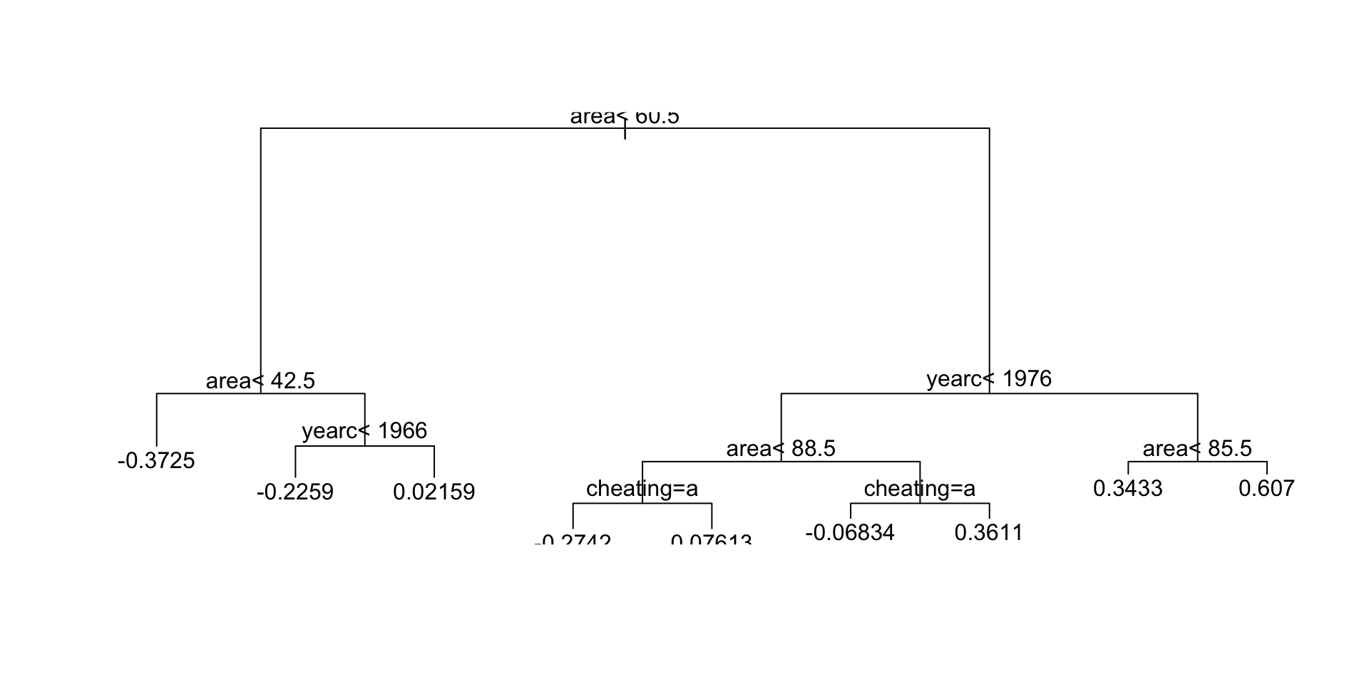
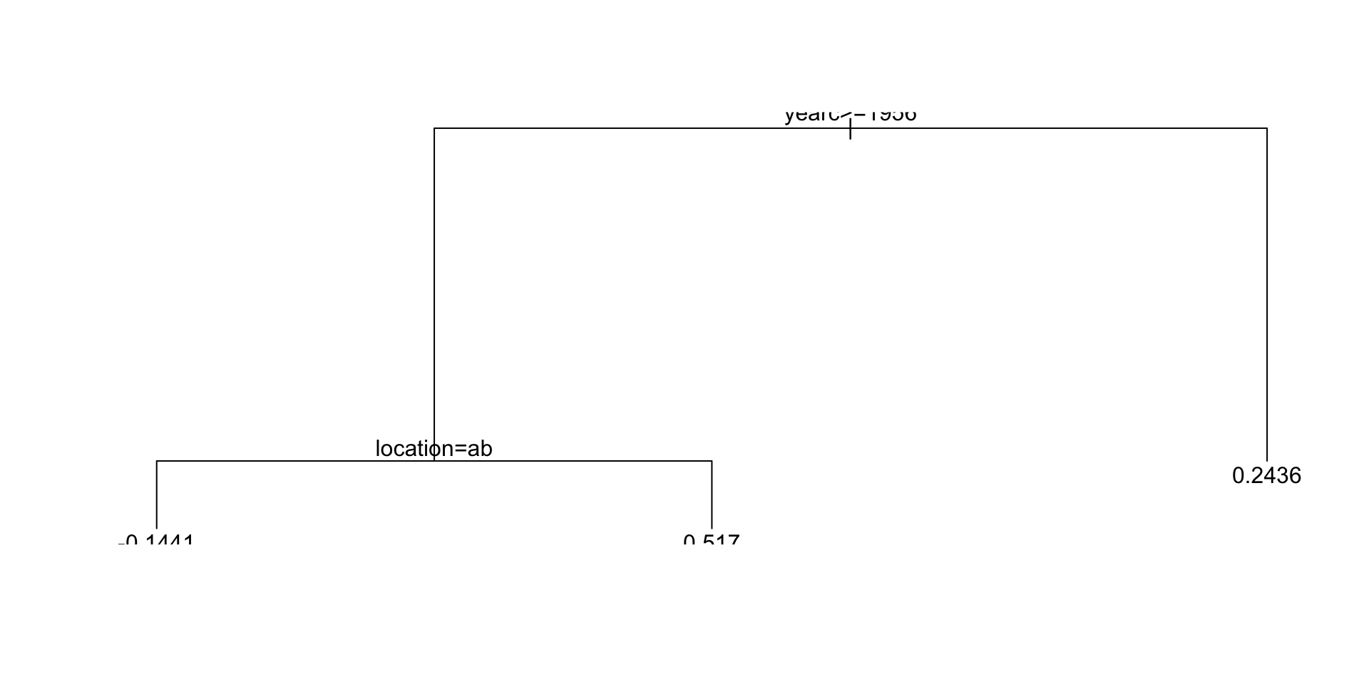
mregtree <- gamlss2(rent~tree(~area+yearc+location+bath+kitchen+cheating)|
                       tree(~area+yearc+location+bath+kitchen+cheating),
                  family=BCTo, data=da, trace=FALSE) 

GAIC(mlinear, madditive, mregtree)

               AIC       df
madditive 38196.79 31.99106
mlinear   38216.10 26.00000
mregtree  38622.27 26.00000

GAIC(mlinear, madditive, mregtree, k=log(dim(rent99)[1]))

               AIC       df
mlinear   38372.97 26.00000
madditive 38389.81 31.99106
mregtree  38779.13 26.00000

Regression Trees (con.)

pp<- specials(mregtree, model = "mu", elements = "model")
plot(pp)
text(pp)

Regression Trees (continue)

pp<-specials(mregtree, model = "sigma", elements = "model")
plot(pp)
text(pp)

Neural Networks (fit)

f <- rent ~ n(~area+yearc+location+bath+kitchen, size=10)|
           n(~area+yearc+location+bath+kitchen, size=3)
mneural <- gamlss2(f,family=BCTo, data=da)

GAMLSS-RS iteration  1: Global Deviance = 38201.2516 eps = 0.290015     
GAMLSS-RS iteration  2: Global Deviance = 38161.604 eps = 0.001037     
GAMLSS-RS iteration  3: Global Deviance = 38156.2641 eps = 0.000139     
GAMLSS-RS iteration  4: Global Deviance = 38155.6106 eps = 0.000017     
GAMLSS-RS iteration  5: Global Deviance = 38155.2744 eps = 0.000008     

gamlss2::GAIC(mlinear, madditive, mneural, mregtree, k=2)

               AIC        df
madditive 38196.79  31.99106
mlinear   38216.10  26.00000
mneural   38375.27 110.00000
mregtree  38622.27  26.00000

gamlss2::GAIC(mlinear, madditive, mneural, mregtree, k=log(dim(rent99)[1]))

               AIC        df
mlinear   38372.97  26.00000
madditive 38389.81  31.99106
mregtree  38779.13  26.00000
mneural   39038.94 110.00000

Neural Networks (plot)

source("~/Dropbox/GAMLSS-development/nnet/plot_NN.R")
 plot(specials(mneural, model = "mu", elements = "model"))

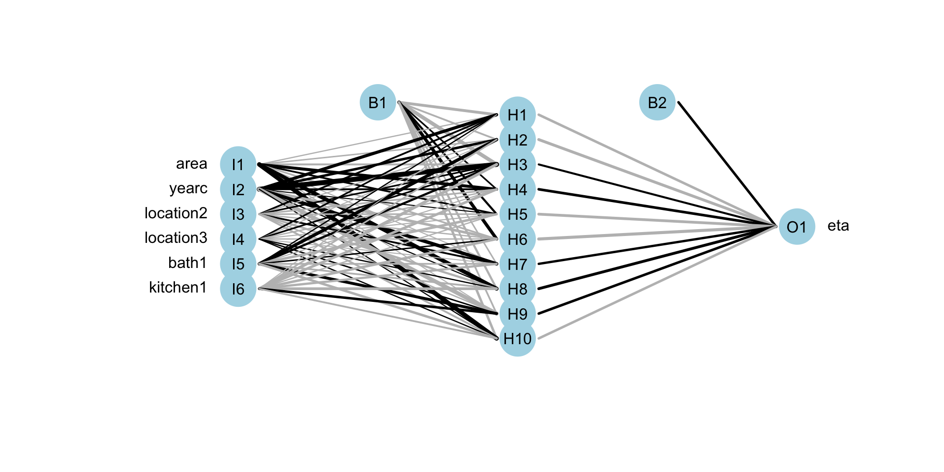
Neural Networks (plot)

source("~/Dropbox/GAMLSS-development/nnet/plot_NN.R")
plot(specials(mneural, model = "sigma", elements = "model"))

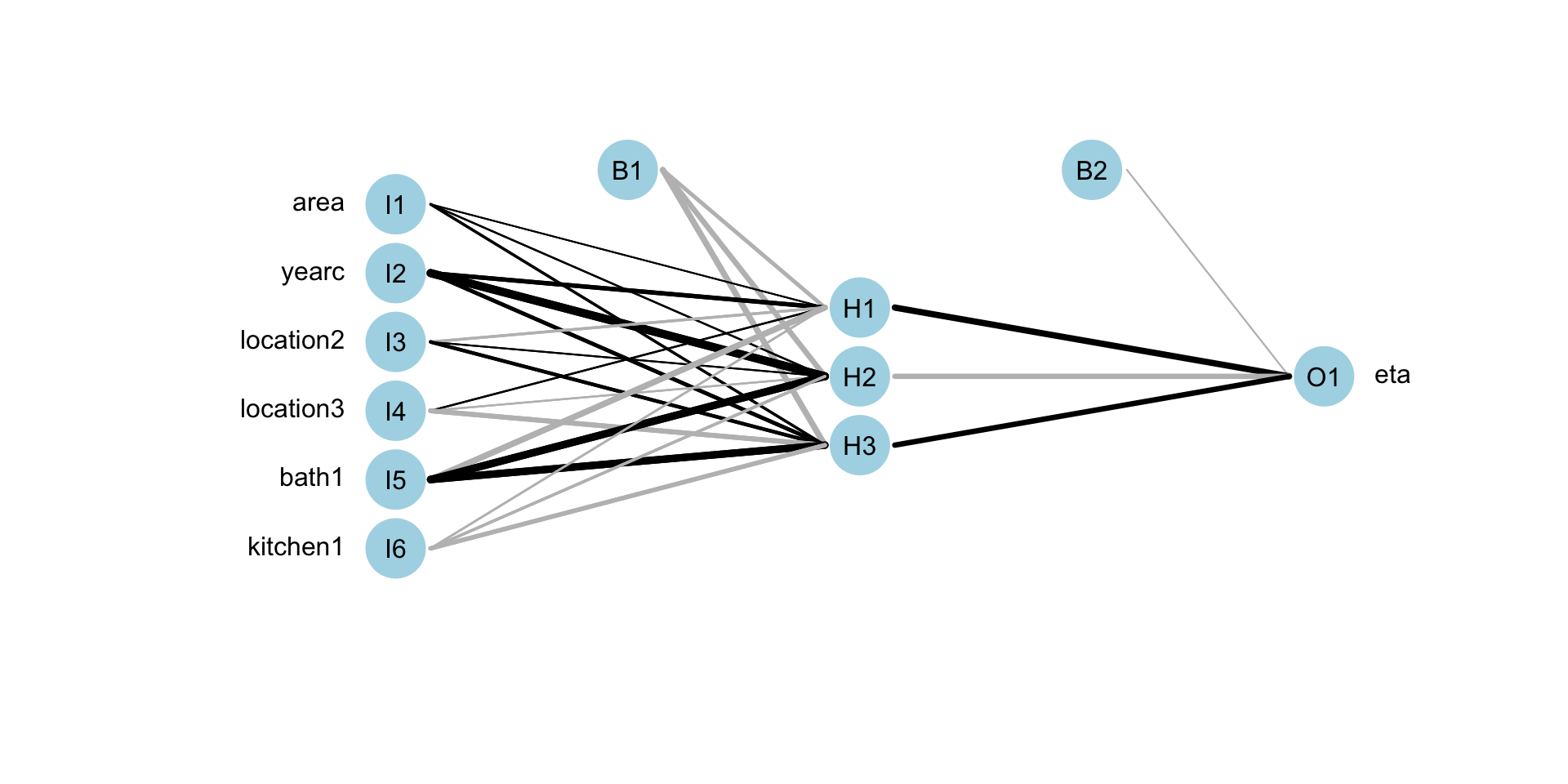
random forest

f <- rent ~ cf(~area+yearc+location+bath+kitchen)|    cf(~area+yearc+location+bath+kitchen)
mcf <- gamlss2(f,family=BCTo, data=da)

GAMLSS-RS iteration  1: Global Deviance = 38466.2361 eps = 0.285090     
GAMLSS-RS iteration  2: Global Deviance = 38312.7521 eps = 0.003990     
GAMLSS-RS iteration  3: Global Deviance = 38307.7194 eps = 0.000131     
GAMLSS-RS iteration  4: Global Deviance = 38306.3367 eps = 0.000036     
GAMLSS-RS iteration  5: Global Deviance = 38306.1885 eps = 0.000003     

gamlss2::GAIC(mlinear, madditive, mneural, mregtree, mcf, k=2)

               AIC        df
madditive 38196.79  31.99106
mlinear   38292.62  19.00000
mneural   38380.62 110.00000
mregtree  38622.27  26.00000
mcf       38714.19 204.00000

LASSO-RIDGE

In gamlss2 there are the functions;

• la() which fit the model using a modified smoothing technique

• lasso() which connects gamlss2 and glmnet

  • the glmnet provides elastic net estimation with alpha=1 equal to lasso and alpha=0 equal to ridge regression

  • the glmnet do not fit a single model but provides the path of all possible models

  • in gamlss2 the model is selected using BIC

LASSO

    area    yearc location     bath  kitchen cheating 
     132       68        3        2        2        2 
 100 % of data are saved, 
that is, 3082 observations. 

    area    yearc location     bath  kitchen cheating 
     132       68        3        2        2        2 

GAMLSS-RS iteration  1: Global Deviance = 38208.7594 eps = 0.289875     
GAMLSS-RS iteration  2: Global Deviance = 38173.0959 eps = 0.000933     
GAMLSS-RS iteration  3: Global Deviance = 38171.6335 eps = 0.000038     
GAMLSS-RS iteration  4: Global Deviance = 38171.2781 eps = 0.000009     

               AIC        df
madditive 38132.81  31.99106
mneural   38155.27 110.00000
mlinear   38164.10  26.00000
bnet      38171.28  24.00000
mcf       38306.19 204.00000
mregtree  38570.27  26.00000

LASSO 1

Call:
gamlss2(formula = fnet1, data = da, family = BCTo)
---
Family: BCTo 
Link functions: mu = log, sigma = log, nu = identity, tau = log
*--------
Coefficients:
                   Estimate Std. Error t value Pr(>|t|)    
mu.(Intercept)     6.073499   0.007714  787.37   <2e-16 ***
sigma.(Intercept) -1.339268   0.007751 -172.79   <2e-16 ***
nu.(Intercept)     0.682562   0.039437   17.31   <2e-16 ***
tau.(Intercept)    3.072434   0.061779   49.73   <2e-16 ***
---
Signif. codes:  0 '***' 0.001 '**' 0.01 '*' 0.05 '.' 0.1 ' ' 1
---
Smooth terms:
    mu.lasso(~area+area2+area3+yearc+yearc2+yearc3+bath1+cheating0+kitchen1+location1+location2)
edf                                                                                           12
    sigma.lasso(~area+area2+area3+yearc+yearc2+yearc3+bath1+cheating0+kitchen1+location1+location2)
edf                                                                                               8
*--------
n = 3082 df =  24 res.df =  3058
Deviance = 38171.2781 Null Dev. Red. = 6.16%
AIC = 38219.2781 elapsed =  0.77sec

LASSO 2

 (Intercept)         area        area2        area3        yearc       yearc2 
 0.170078437  0.244928458 -0.033422433  0.004850439  0.138919707  0.062595342 
      yearc3        bath1    cheating0     kitchen1    location1    location2 
-0.013271475  0.060201306 -0.338518720  0.111794049 -0.222495637 -0.131310857 

 (Intercept)         area        area2        area3        yearc       yearc2 
 0.044503278  0.019210761 -0.013455170  0.005293646 -0.249616969  0.000000000 
      yearc3        bath1    cheating0     kitchen1    location1    location2 
 0.055728860  0.000000000  0.212985531  0.000000000 -0.059687857  0.000000000 

NULL

Principal Componet Regression

• functions pc() and pcr() in gamlss.foreach package for gamlss

• PCR is non implemented for gamlss2 yet

summary

Table 1: Summary of properties of the machine learning algorithms

ML Models	coef. s.e.	stand. of x’s	algo. stab., speed, conv.	non-linear terms	inter- actions	data type	auto sele-ction	interpre- tation
linear	yes	no	yes, fast, v.good	poly	declare	\(n>r\)	no	v. easy
additive	no	no	yes, slow, good	smooth	declare	\(n>r\)	no	easy
RT	no	no	no, slow, bad	trees	auto	\(n>r\)??	yes	easy

summary (continue)

Table 2: Summary of properties of the machine learning algorithms

ML Models	coef. s.e.	stand. of x’s	algo. stab., speed, conv.	non-linear terms	inter- actions	data type	auto sele-ction	interpre- tation
NN	no	0 to 1	no, \(\,\,\) ok, \(\,\,\) ok	auto	auto	both?	yes	v. hard
RF	no	no	no, slow, slow	YES	no	both	auto	hard
LASSO	no	yes	yes, fast, good	poly	declare	both	auto	easy

summary (continue)

Table 3: Summary of properties of the machine learning algorithms

ML Models	coef. s.e.	stand. of x’s	algo. stab., speed, conv.	non-linear terms	inter- actions	data type	auto sele-ction	interpre- tation
Boost	no	no	yes, fast, good	smooth trees	declare	\(n<<r\)	yes	easy
MCMC	yes	no	good, ok, \(\,\,\) ok	smooth	declare	\(n>r\)	no	easy
PCR	yes	yes	yes, fast, good	poly	declare	both	auto	hard

end

back to the index

The Books