Statistical models
“all models are wrong but some are useful”.
– George Box
Models should be parsimonious
Models should be fit for purpose and able to answer the question at hand
Statistical models have a stochastic component
All models are based on assumptions .
A common theme in the following scientific subjects; statistical analysis ; statistical inference ; statistical modelling ; machine learning ; statistical learning ; data mining ; information harvesting ; information discovery ; knowledge extraction ; data analytics , is data .
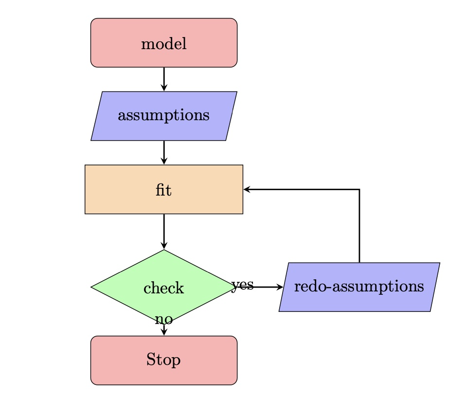
Model circle
Regression
\[
X \stackrel{\textit{M}(\theta)}{\longrightarrow} Y
\] \(y\) : targer , the y or the dependent variable\(X\) : explanatory , features , x’s or independent variables or terms
Linear Model
\[
\begin{equation}
y_i= b_0 + b_1 x_{1i} + b_2 x_{2i}, \ldots, b_p x_{pi}+ \epsilon_i
\end{equation}
\qquad(1)\]
the model \(M(\theta)\) is linear, and there are \(n\) observations for \(i=1,2,\ldots,n\) .
Linear Model
\[
\begin{split}
y_i & \stackrel{\small{ind}}{\sim } & {N}(\mu_i, \sigma) \nonumber \\
\mu_i &=& b_0 + b_1 x_{1i} + b_2 x_{2i}, \ldots, b_p x_{pi}
\end{split}
\qquad(2)\]
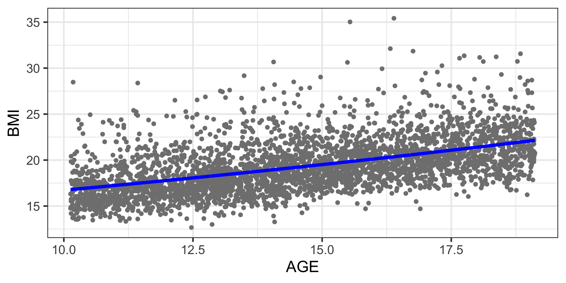
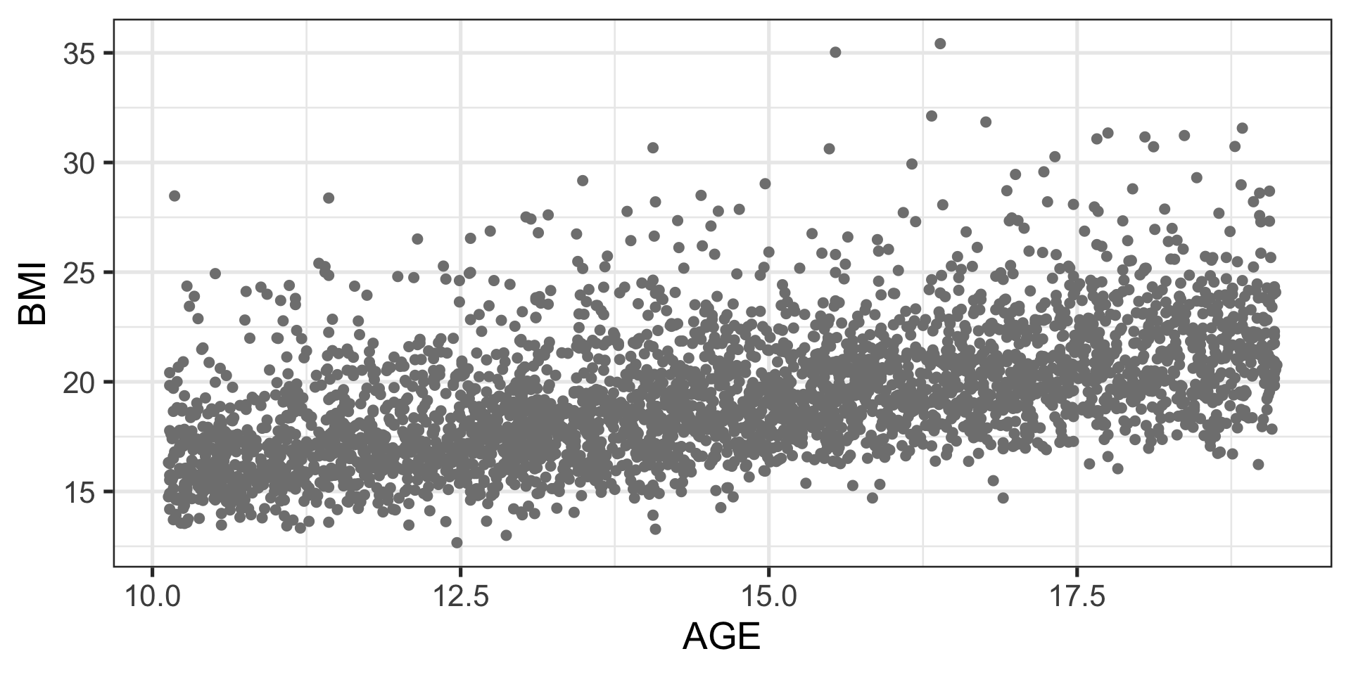
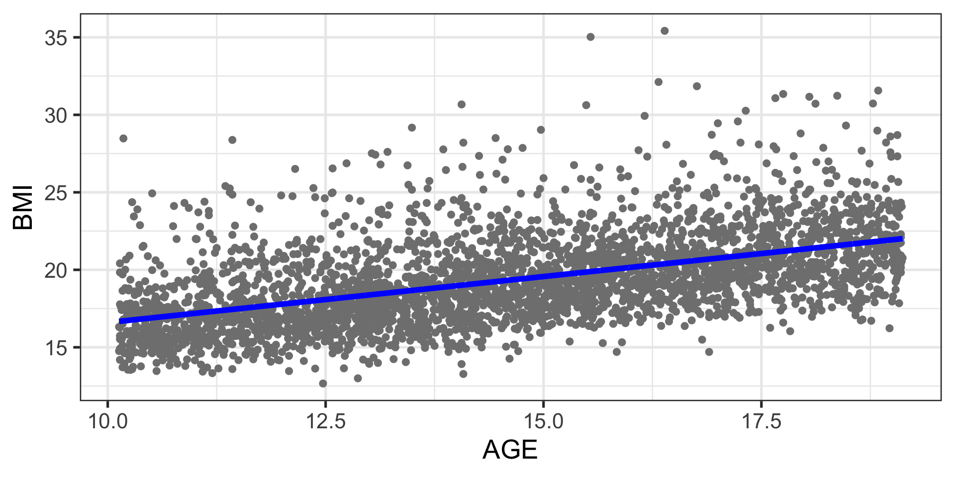
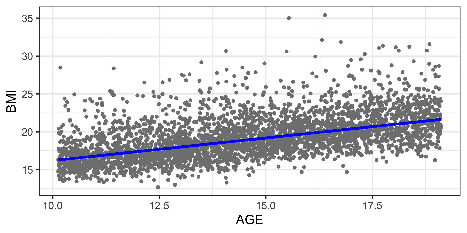
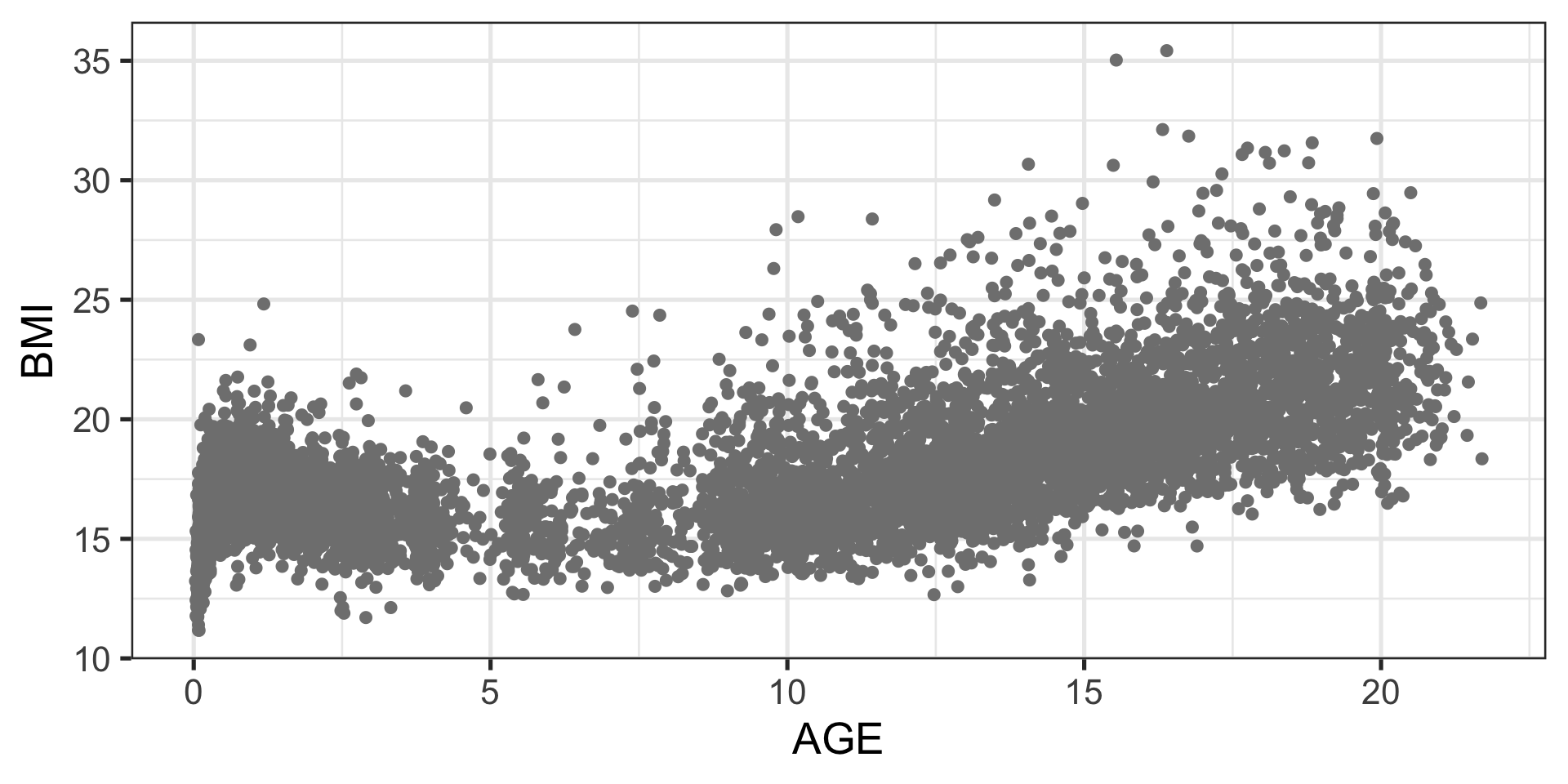
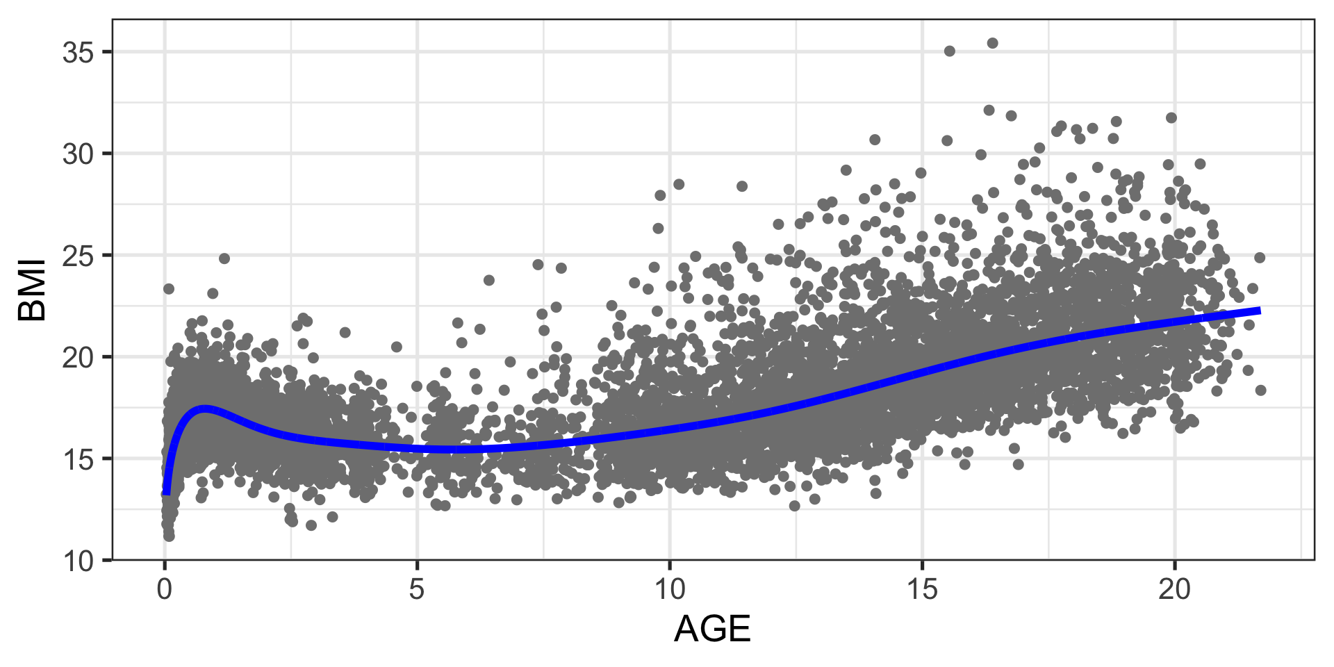
Example: BMI data
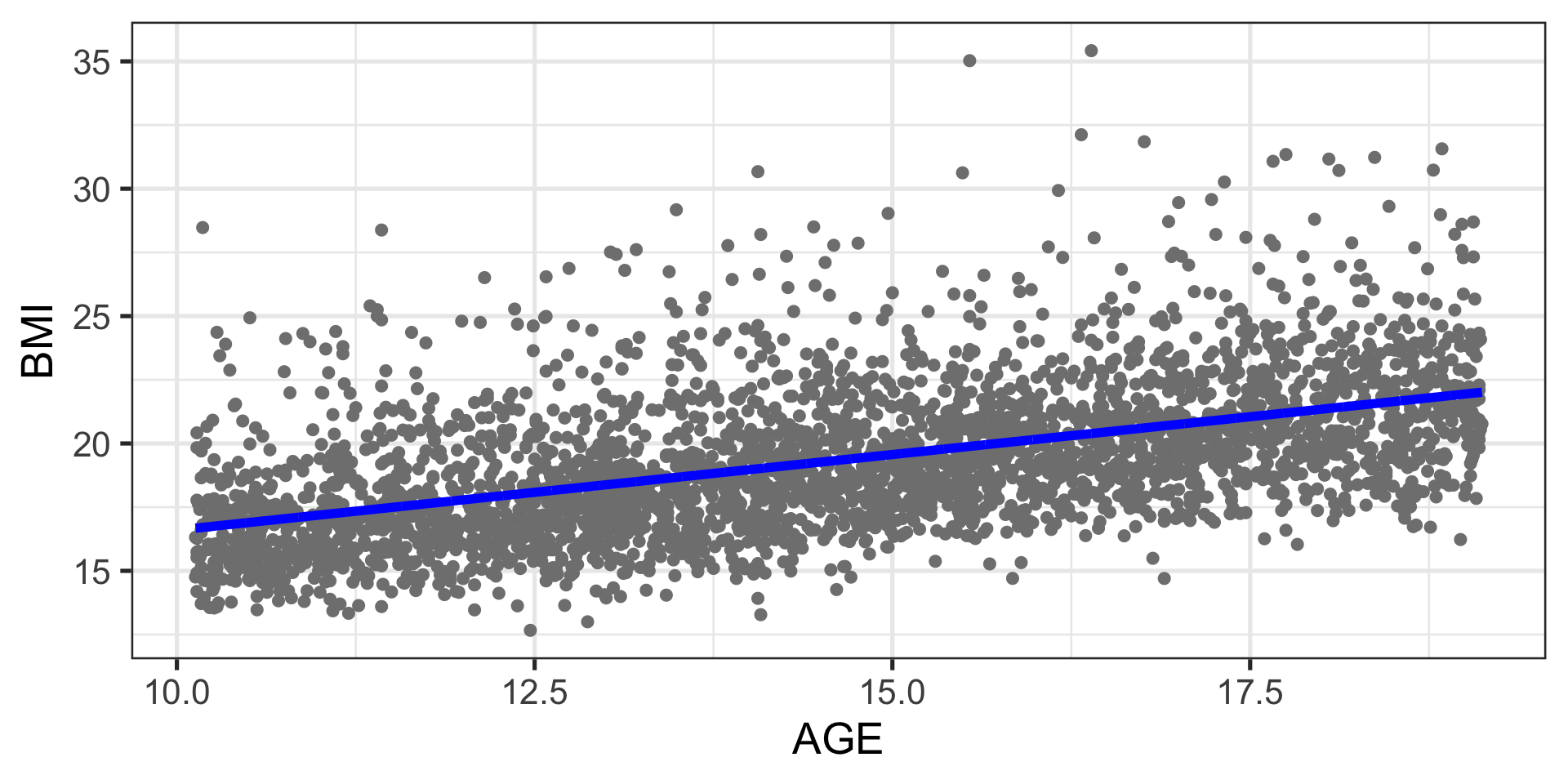
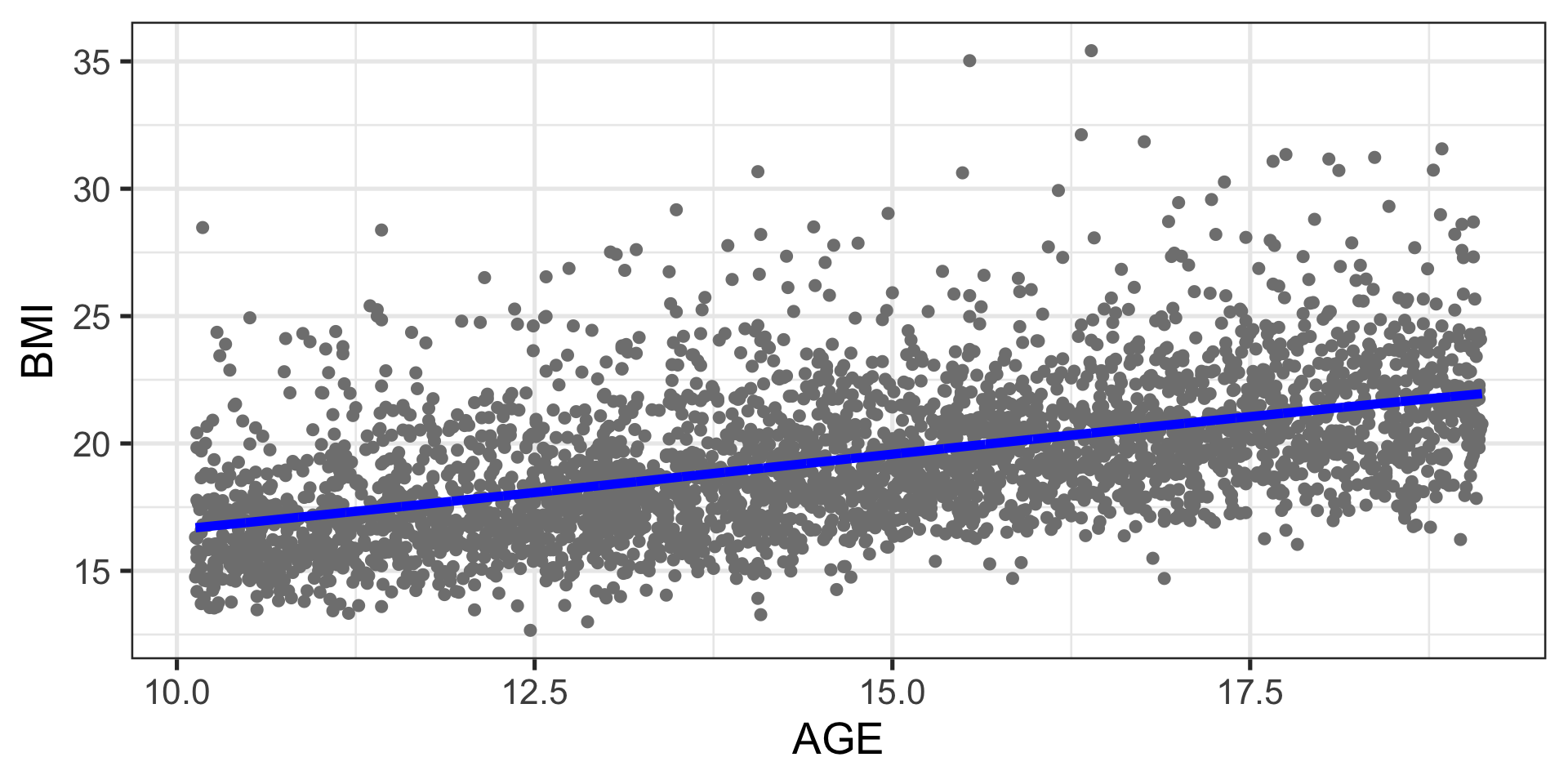
Example: BMI fitted model
Additive Models
\[
\begin{split}
y_i & \stackrel{\small{ind}}{\sim } & {N}(\mu_i, \sigma) \nonumber \\
\mu_i &=& b_0 + s_1(x_{1i}) + s_2(x_{2i}), \ldots, s_p(x_{pi})
\end{split}
\qquad(3)\]
Example: additive fitted model
Machine Learning Models
\[\begin{split}
y_i & \stackrel{\small{ind}}{\sim }& {N}(\mu_i, \sigma) \nonumber \\
\mu_i &=& ML(x_{1i},x_{2i}, \ldots, x_{pi})
\end{split}
\qquad(4)\]
Example: neural networks
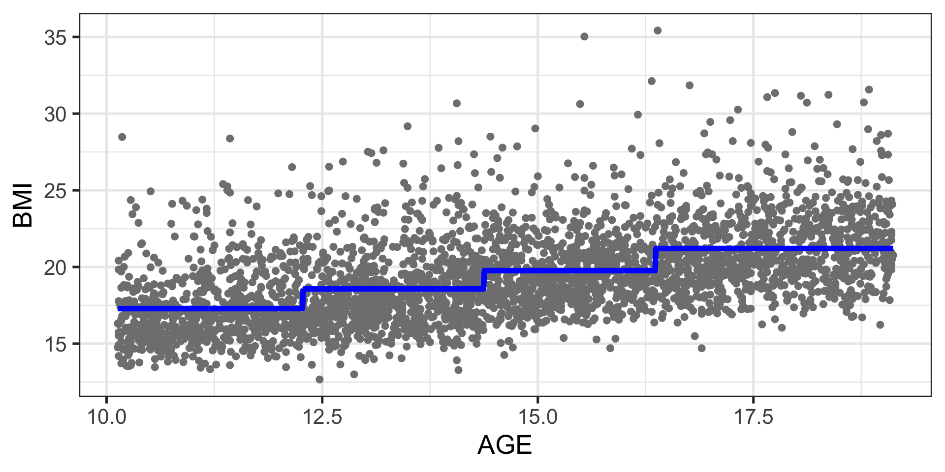
Example: regression tree
Generalised Linear Models
\[\begin{split}
y_i & \stackrel{\small{ind}}{\sim }& {E}(\mu_i, \phi) \nonumber \\
g(\mu_i) &=& b_0 + b_1 x_{1i} + b_2 x_{2i}, \ldots, b_p x_{pi}
\end{split}
\qquad(5)\]
Example: conclusion
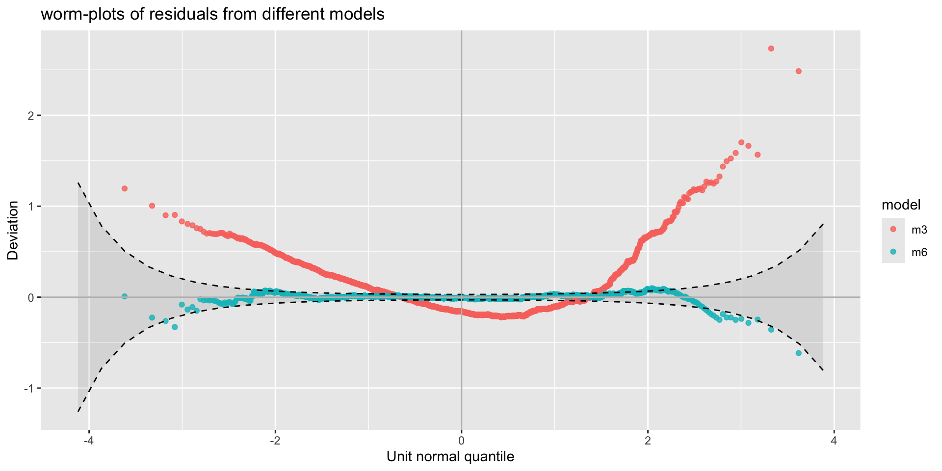
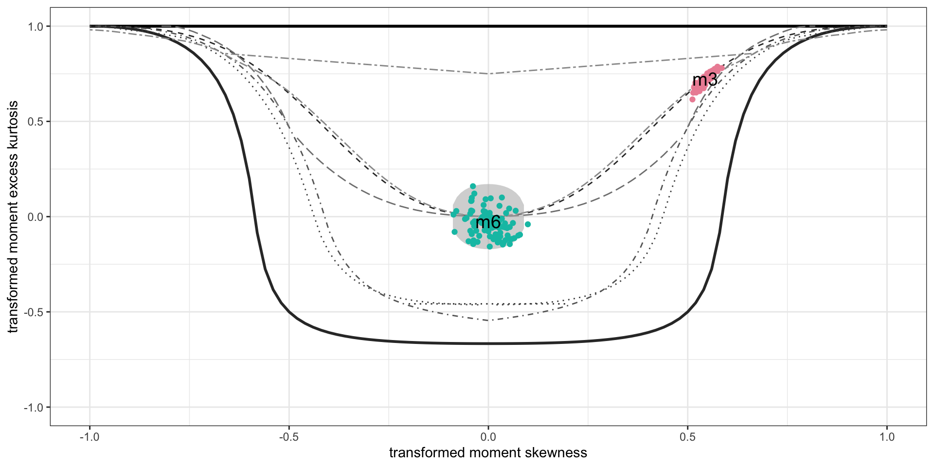
the mean of the response is fitted fine with the linear model but the distribution is not
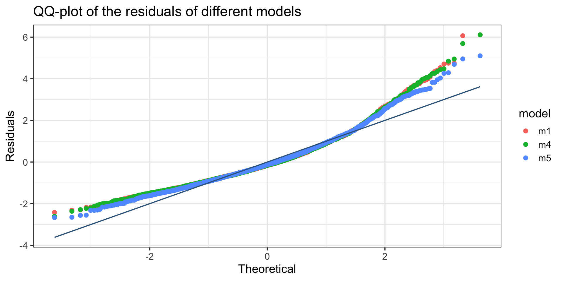
the distribution (implicit Normal) is not-adequate
even the explicit Gamma distribution of the GLM is not-adequate
therefore if we are interested on a statistic different from the mean we need something extra.
Distributional regression
Distributional regression
\[
X \stackrel{\textit{M}(\boldsymbol{\theta})}{\longrightarrow} D\left(Y|\boldsymbol{\theta}(\textbf{X})\right)
\]
All parameters \(\boldsymbol{\theta}\) could functions of the explanatory variables \(\boldsymbol{\theta}(\textbf{X})\) .
\(D\left(Y|\boldsymbol{\theta}(\textbf{X})\right)\) can be any \(k\) parameter distribution
Generalised Additive models for Location Scale and Shape
\[\begin{split}
y_i & \stackrel{\small{ind}}{\sim }& {D}( \theta_{1i}, \ldots, \theta_{ki}) \nonumber \\
g(\theta_{1i}) &=& b_{10} + s_1({x}_{1i}) + \ldots, s_p({x}_{pi}) \nonumber\\
\ldots &=& \ldots \nonumber\\
g({\theta}_{ki}) &=& b_0 + s_1({x}_{1i}) + \ldots, s_p({x}_{pi})
\end{split}
\qquad(6)\]
GAMLSS + ML
\[\begin{split}
y_i & \stackrel{\small{ind}}{\sim }& {D}( \theta_{1i}, \ldots, \theta_{ki}) \nonumber \\
g({\theta}_{1i}) &=& {ML}_1({x}_{1i},{x}_{2i}, \ldots, {x}_{pi}) \nonumber \\
\ldots &=& \ldots \nonumber\\
g({\theta}_{ki}) &=& {ML}_1({x}_{1i},{x}_{2i}, \ldots, {x}_{pi})
\end{split}
\qquad(7)\]
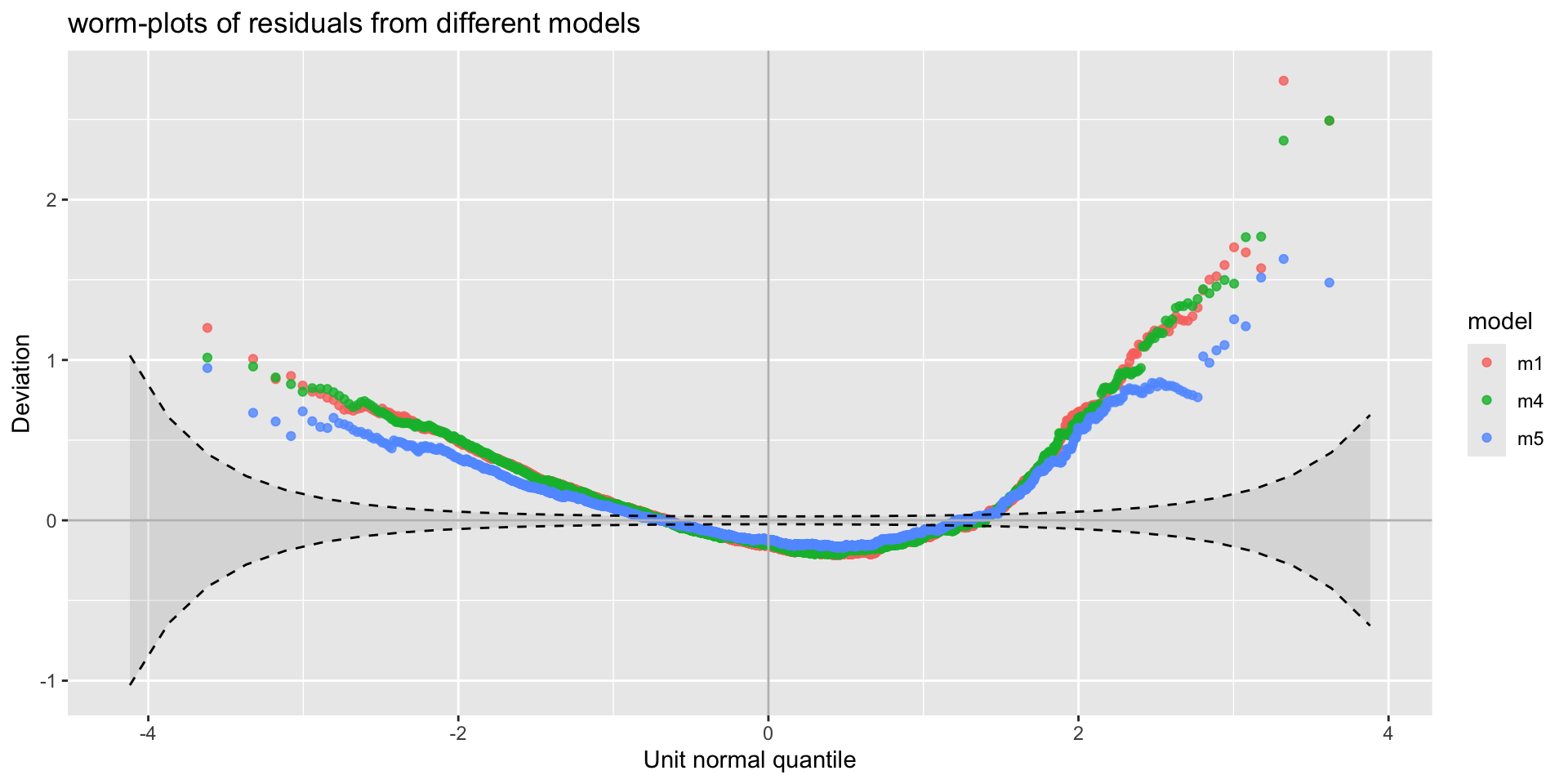
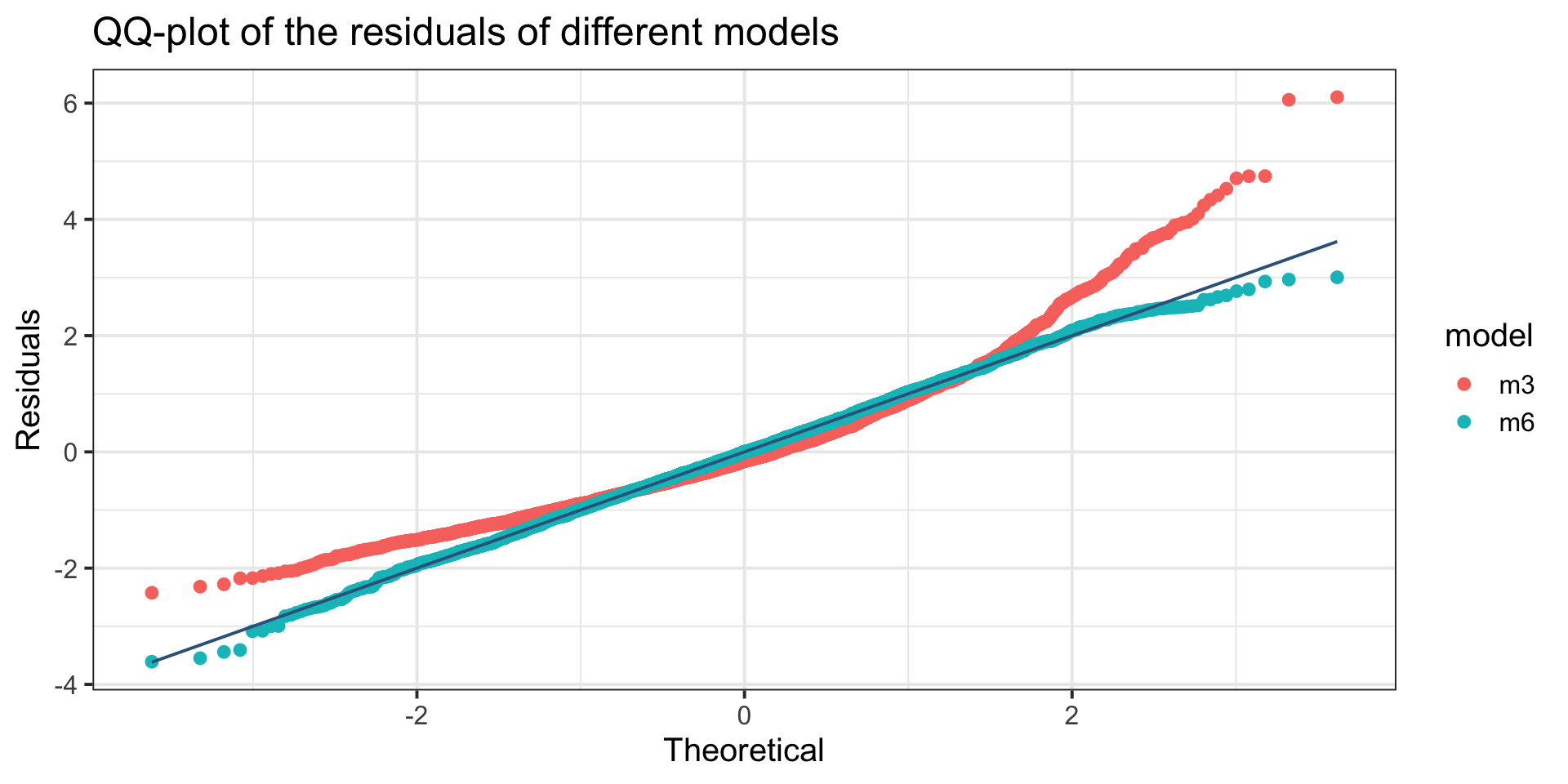
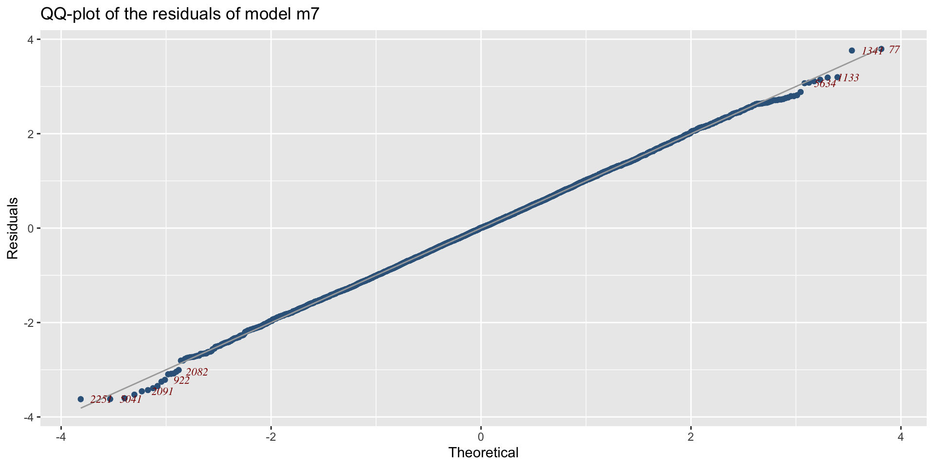
Example: diagnostics
QQ-plot, Gamma, m3, against BCT model, m6.
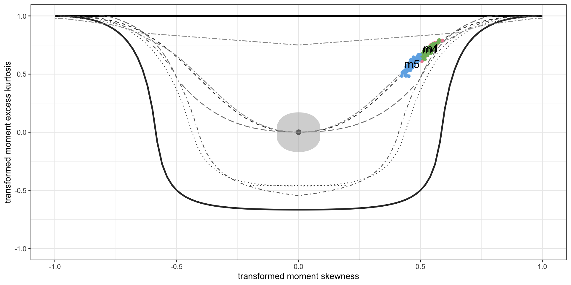
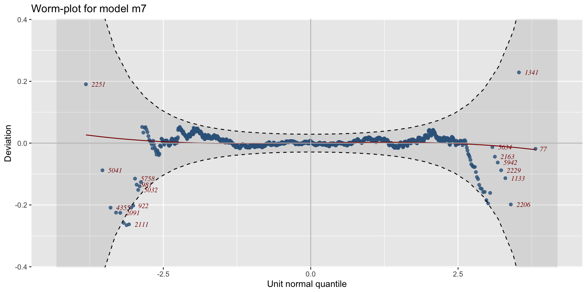
Example: diagnostics 3
Bucket-plot, Gamma, m3, against BCT model, m6.
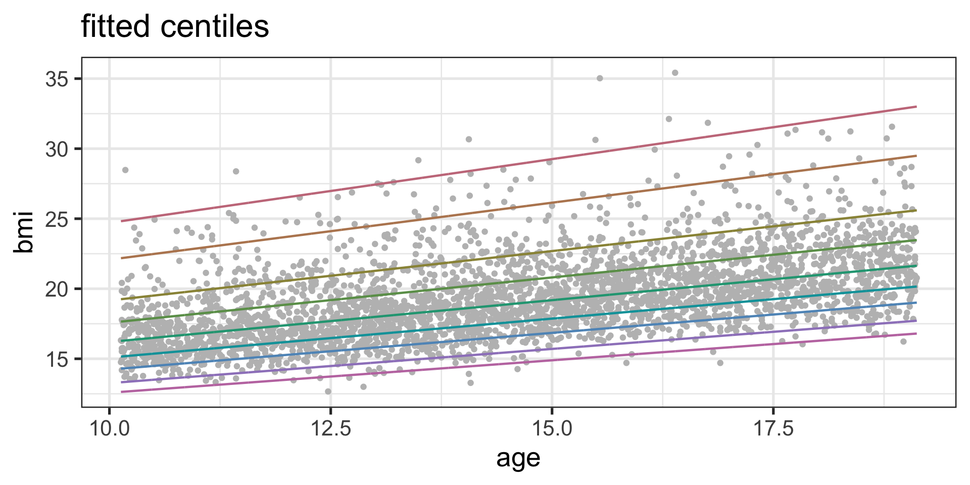
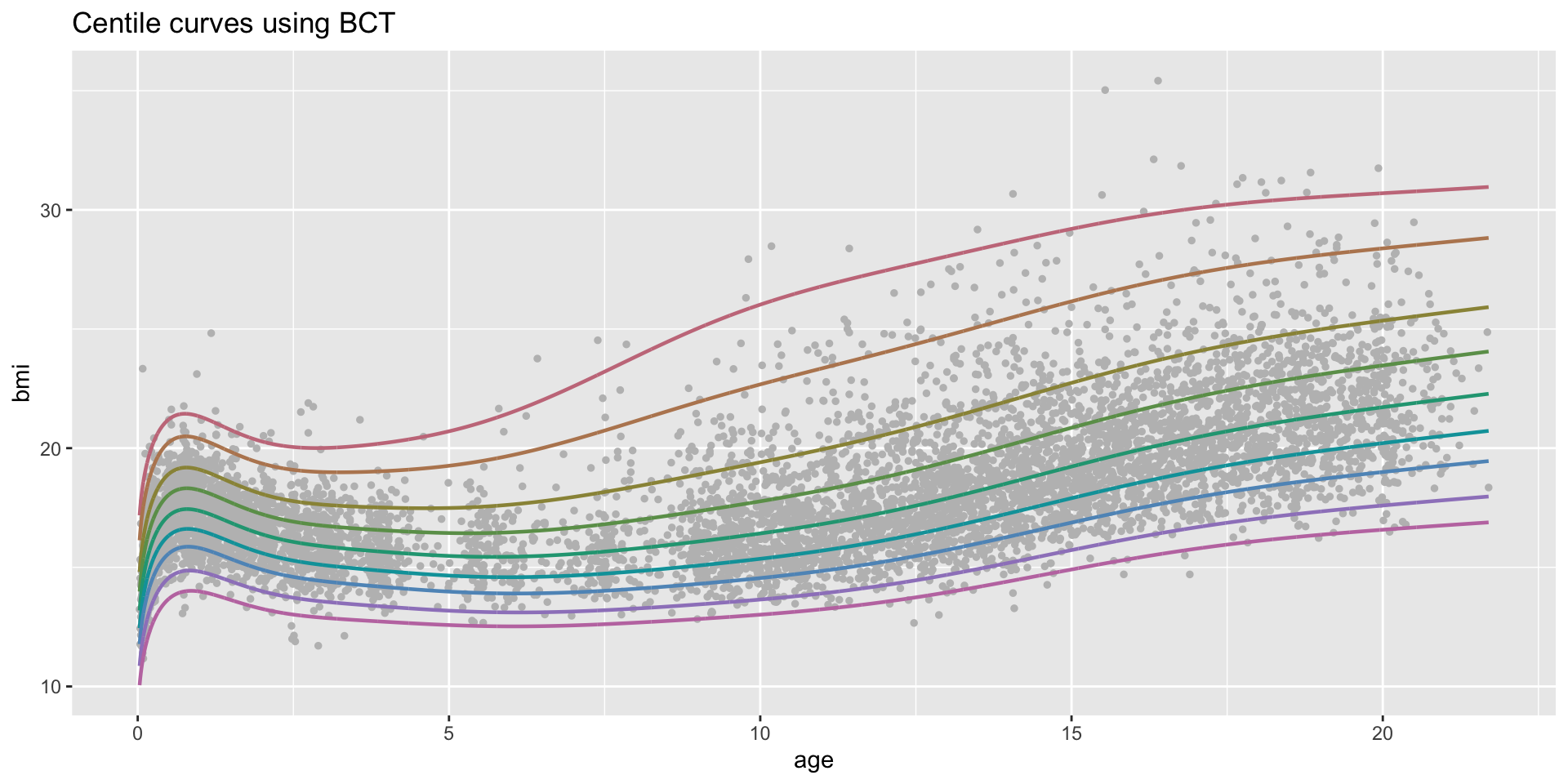
Fitted Centiles
Figure 1: Centile-plot of the fitted m6 model
The true BMI data
The fitted model
Summary
Distributional assumptions often needed for the response to be fitted properly
In the BMI example above we needed to model all the parameters of the distribution as function of the explanatory variable age.
Those parameters were the location parameter \(\mu\) , the scale parameter, \(\sigma\) , the skewness parameter, \(\nu\) , and the kurtotic parameter \(\tau\)
Machine Learning methods are useful (especially for modelling interactions between variables) but they are not suitable if the interest do not lie in the mean of the distribution.
 The Books