Interpreting models

Mikis Stasinopoulos
Bob Rigby
Fernanda De Bastiani
Gillian Heller
Niki Umlauf

Introduction

  • how to interpreted the effect of a single term into the distribution of the response;
  • how to use the GAMLSS model for prediction.

Interpretation

  • how the information we obtain from the fitted model can be used
flowchart TB
  A[Features.] --> B(Parameters) 
  B --> D[Properties, \n Characteristics]
  D -->  C(Distribution)
  B --> C
Figure 1: How x-variables effecting the properties of the distribution.

graphical Partial effects

  • ceteris paribus (concentate in one term fixing the rest)

  • \(\textbf{x}_j\) denote a single (or maximum two terms)

  • \(\textbf{x}_{-j}\) all the rest so \(\{\textbf{x}_j, \textbf{x}_{-j} \}\) are all terms in the model

  • \(\omega(D)\) the characteristic of the distribution we are interested \({D}(y | \textbf{x}_j , \textbf{x}_{-j}; \boldsymbol{\theta})\) i.e. kurtosis

  • under scenario, \(\textbf{S}[g()]\) ()

  • \[{PE}_{\omega({D})}\left( \textbf{x}_{j} | \textbf{S} \left[ g(\textbf{x}_{-j})\right] \right)\]

Scenarios

  • fixing values of \(\textbf{x}_{-j}\) (mean or median for continuous, level with more number of observations for factors or other possible values of importance)

  • average over values of \(\textbf{x}_{-j}\)

    • Partial Dependence Plots (PDF), \(\textbf{S}\left[ \text{average}(\textbf{x}_{-j})\right]\)
    • Accumulated Local Effects, (ALE), accumulated average local differences
    • Marginal Effects (ME) average over local neighbourhood

Characteristics

  • predictors, \(\eta_{\theta_i}\)

  • parameters, \(\theta_i\)

  • moment, i.e. mean and variance

  • quantiles i.e. median

  • distribution

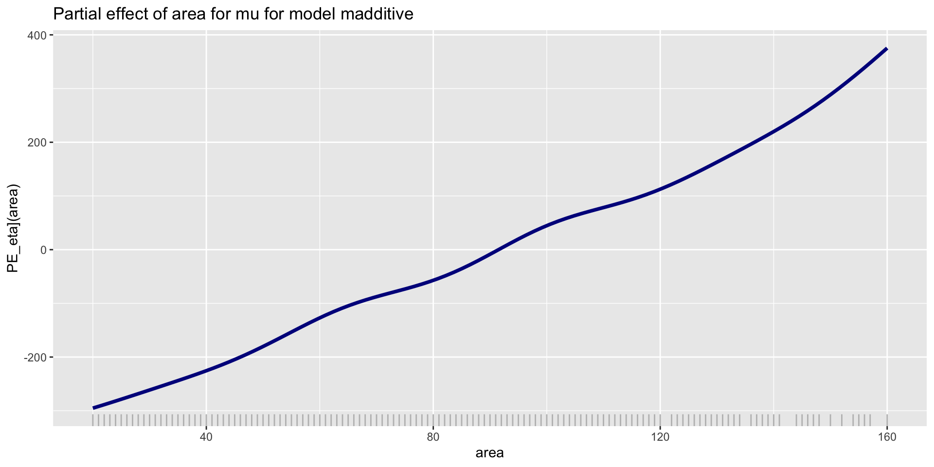
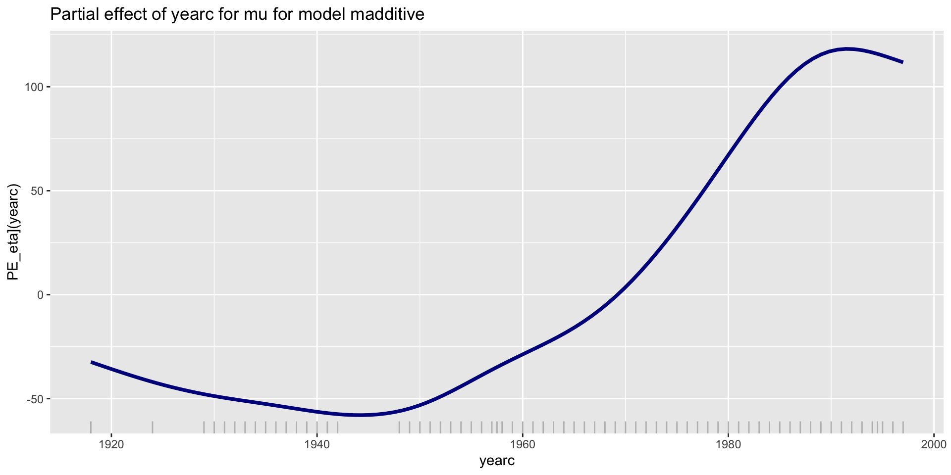
PE-parameter \(\mu\) additive

library(gamlss.ggplots)
pe_param(madditive,"area")
pe_param(madditive,"yearc")

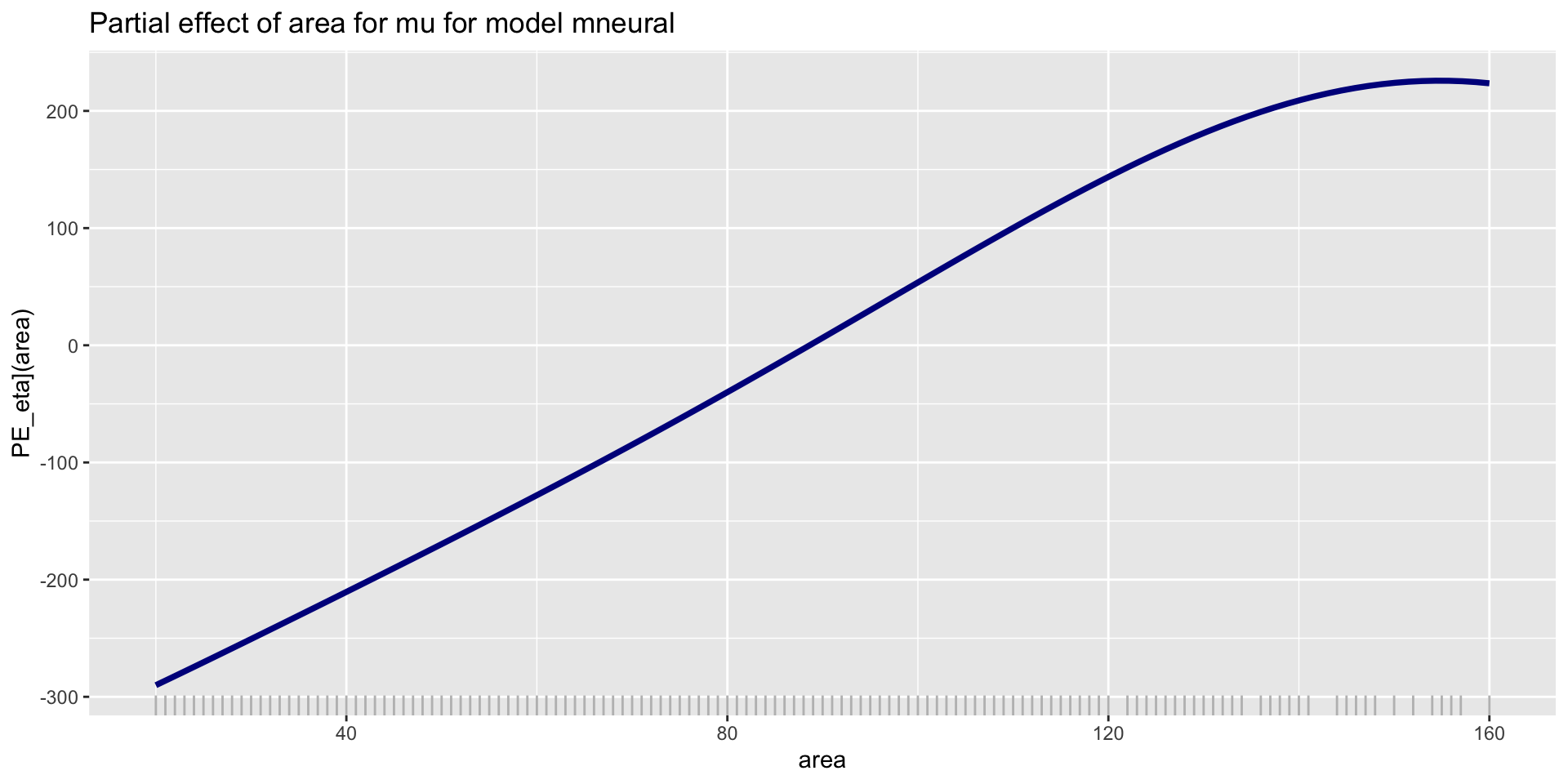
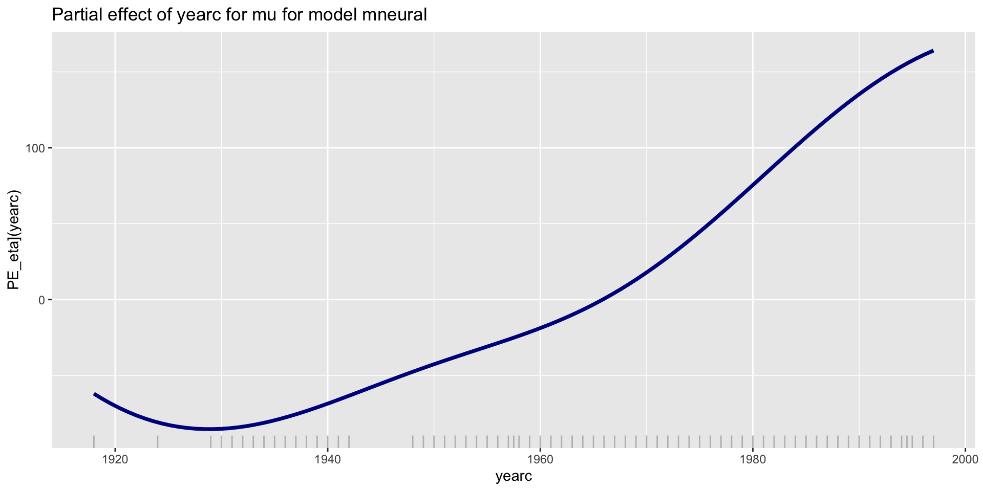
PE-parameter \(\mu\) NN

pe_param(mneural, "area" )
pe_param(mneural, "yearc" )

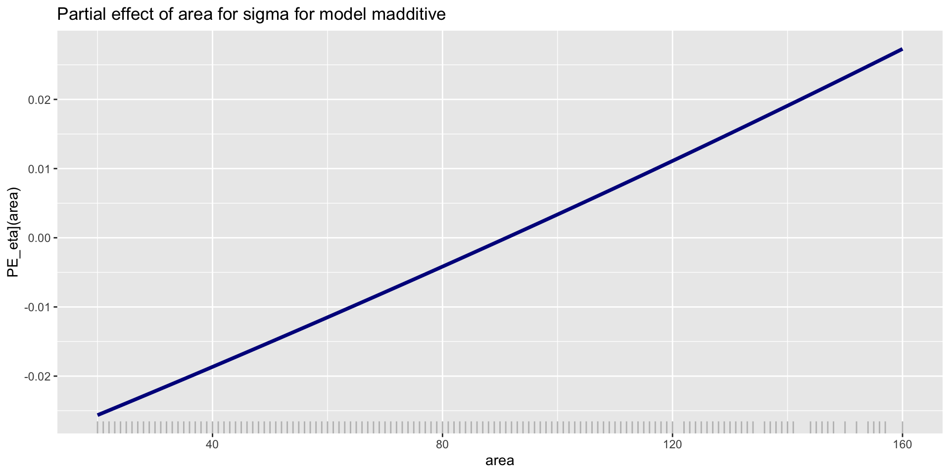
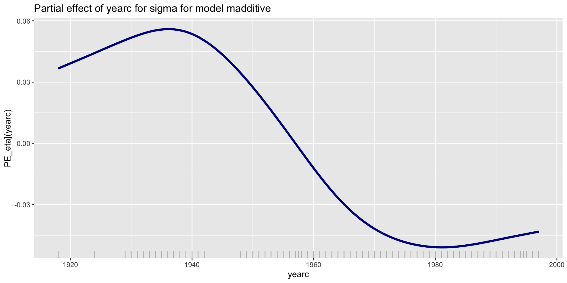
PE; parameter \(\sigma\); additive

pe_param(madditive,"area", parameter="sigma")
pe_param(madditive,"yearc", parameter="sigma")

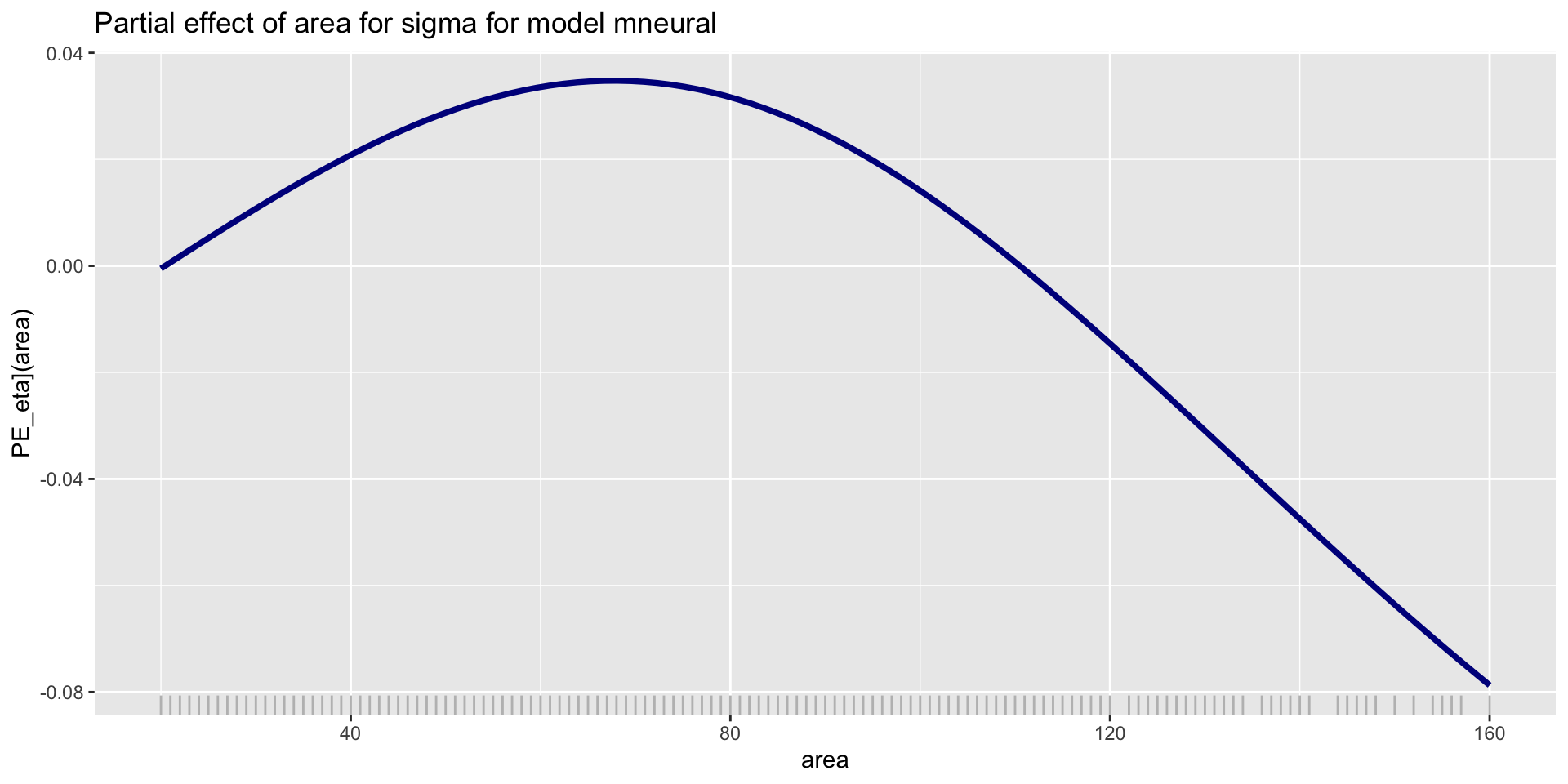
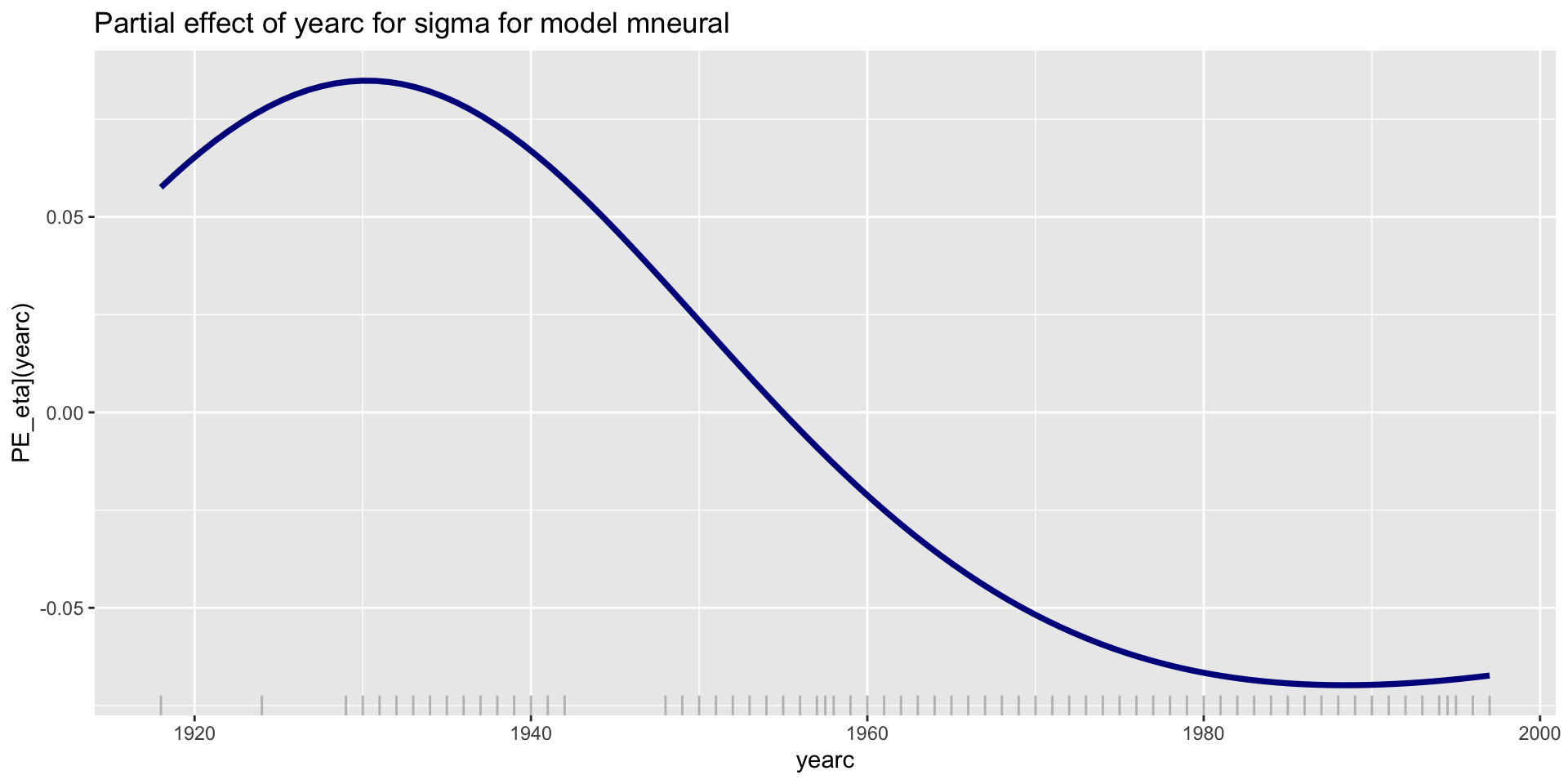
PE; parameter \(\sigma\); NN

pe_param(mneural,"area", parameter="sigma")
pe_param(mneural,"yearc", parameter="sigma")

all terms (additive)

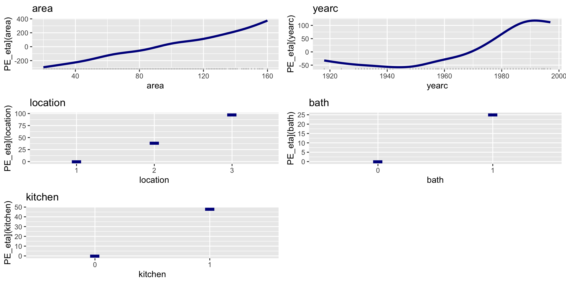
pe_param_grid(madditive,c("area", "yearc",  "location", "bath", "kitchen"))

2 way interactions (additive)

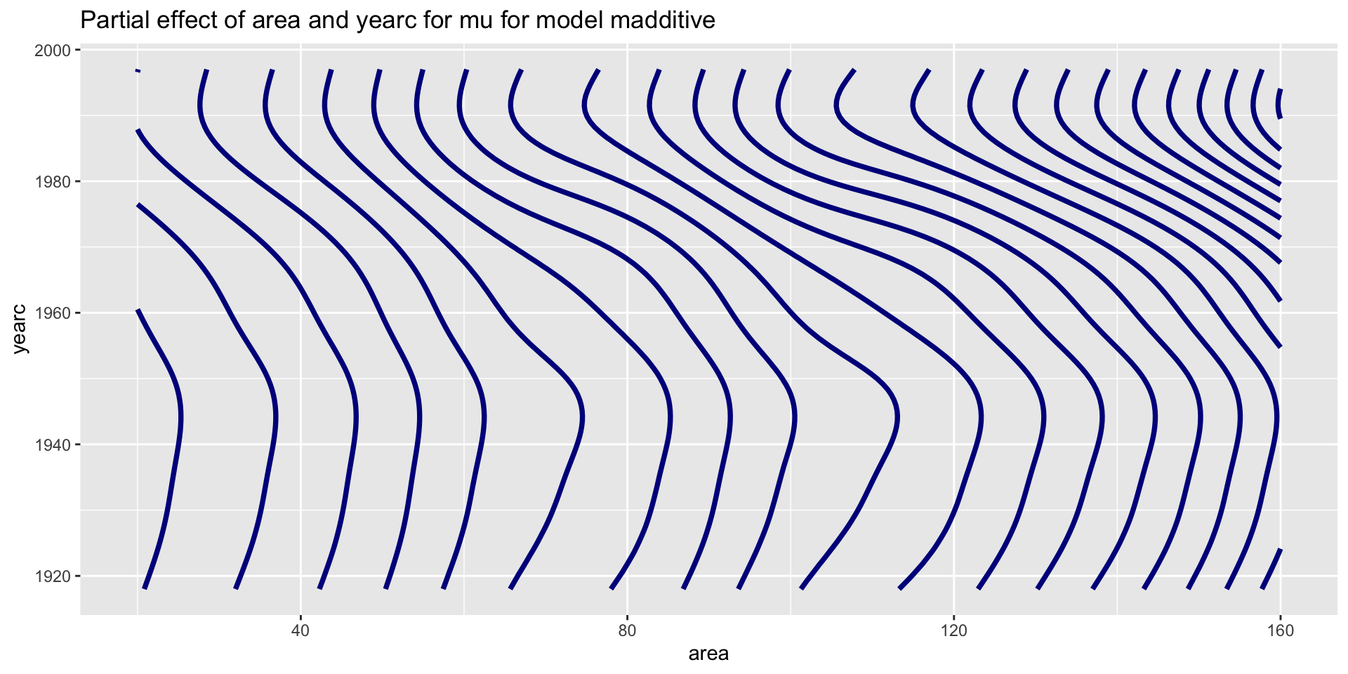
 pe_param(madditive, c("area", "yearc")) 
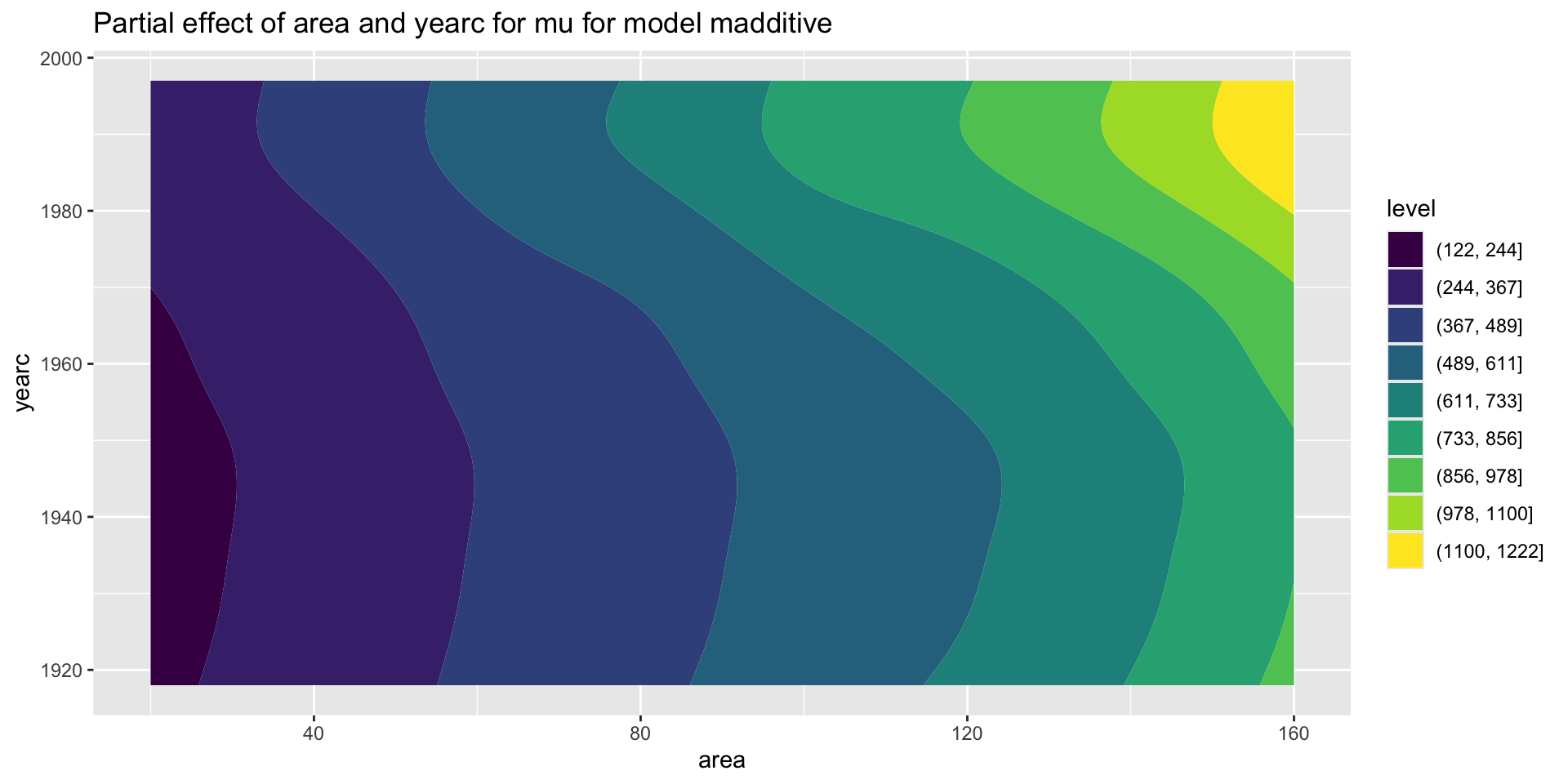
pe_param( madditive, c("area", "yearc"), filled=TRUE) 

pe_pdf

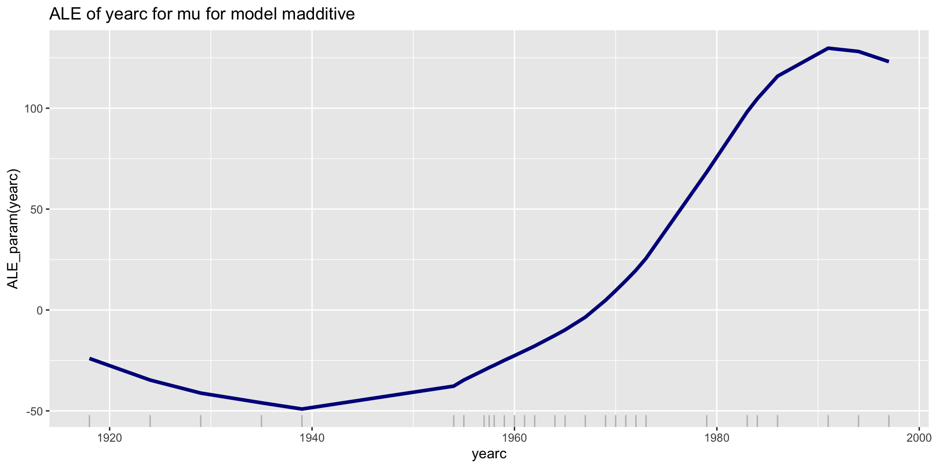
ALE; parameters \(\mu\); Additive

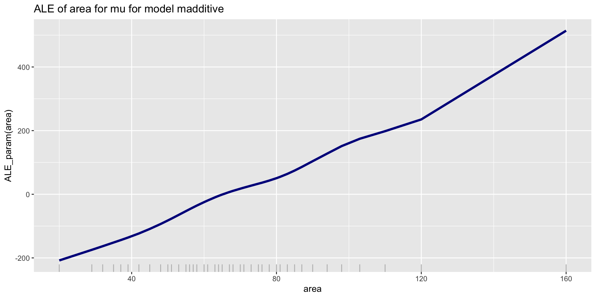
gamlss.ggplots:::ale_param(madditive,"area")
gamlss.ggplots:::ale_param(madditive,"yearc")

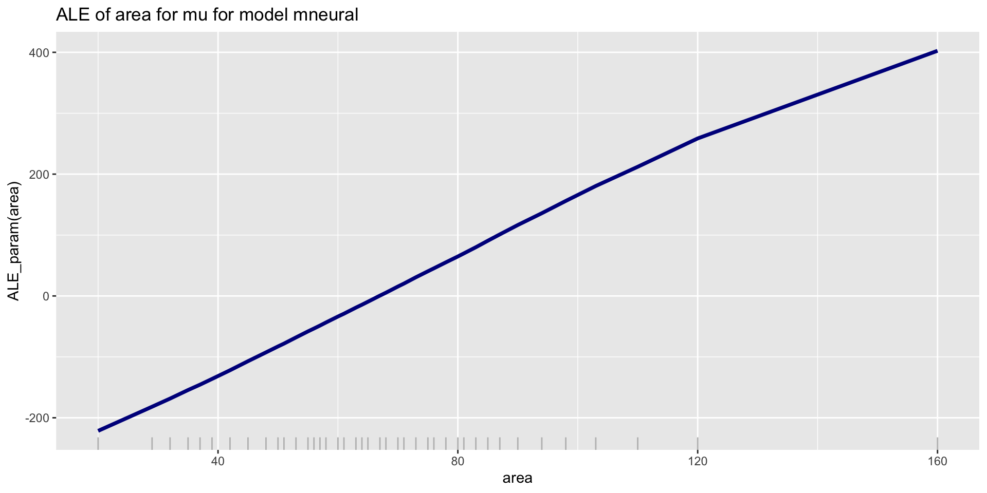
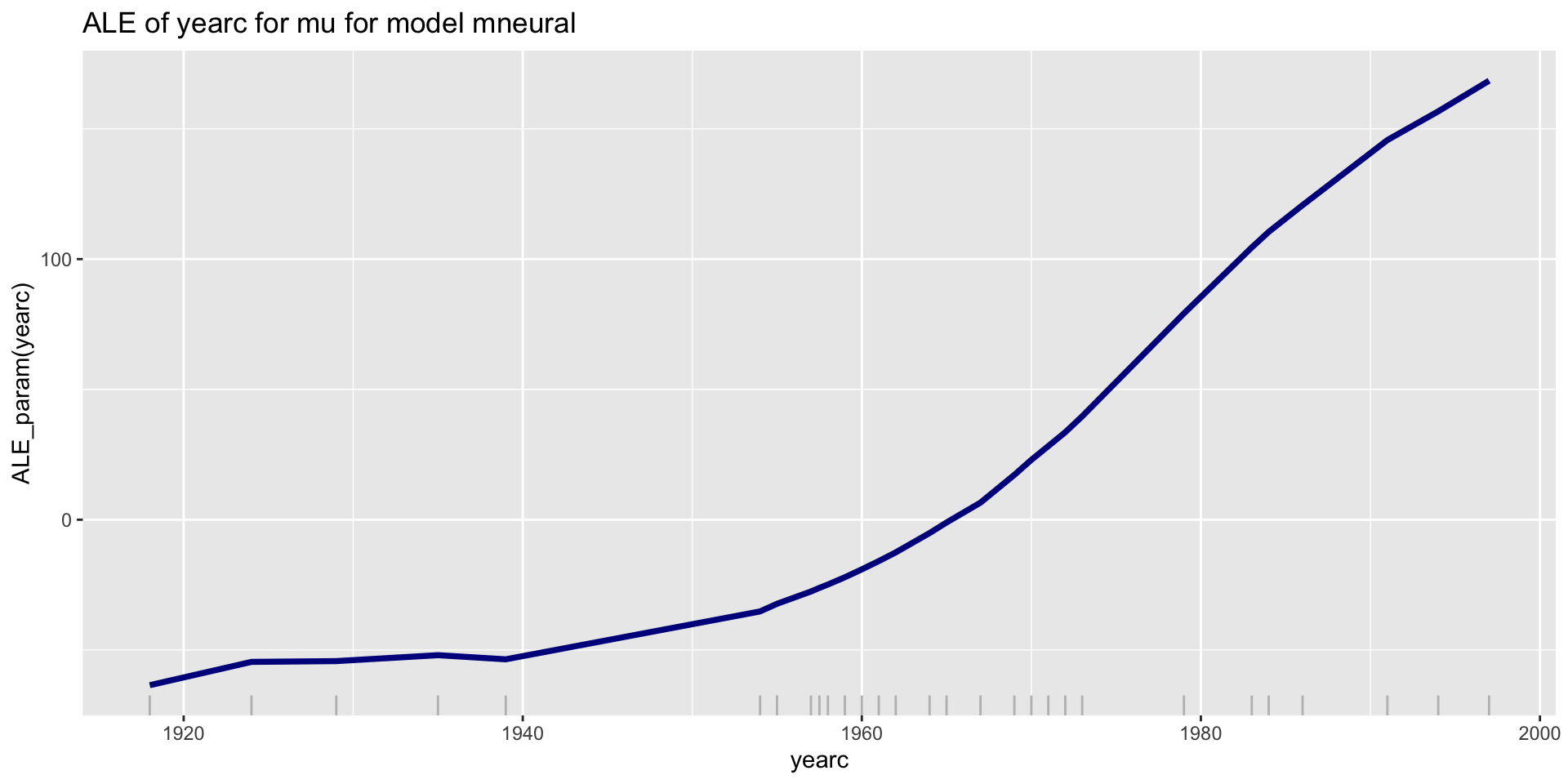
ALE; parameters \(\mu\); NN

gamlss.ggplots:::ale_param(mneural,"area")
gamlss.ggplots:::ale_param(mneural,"yearc")

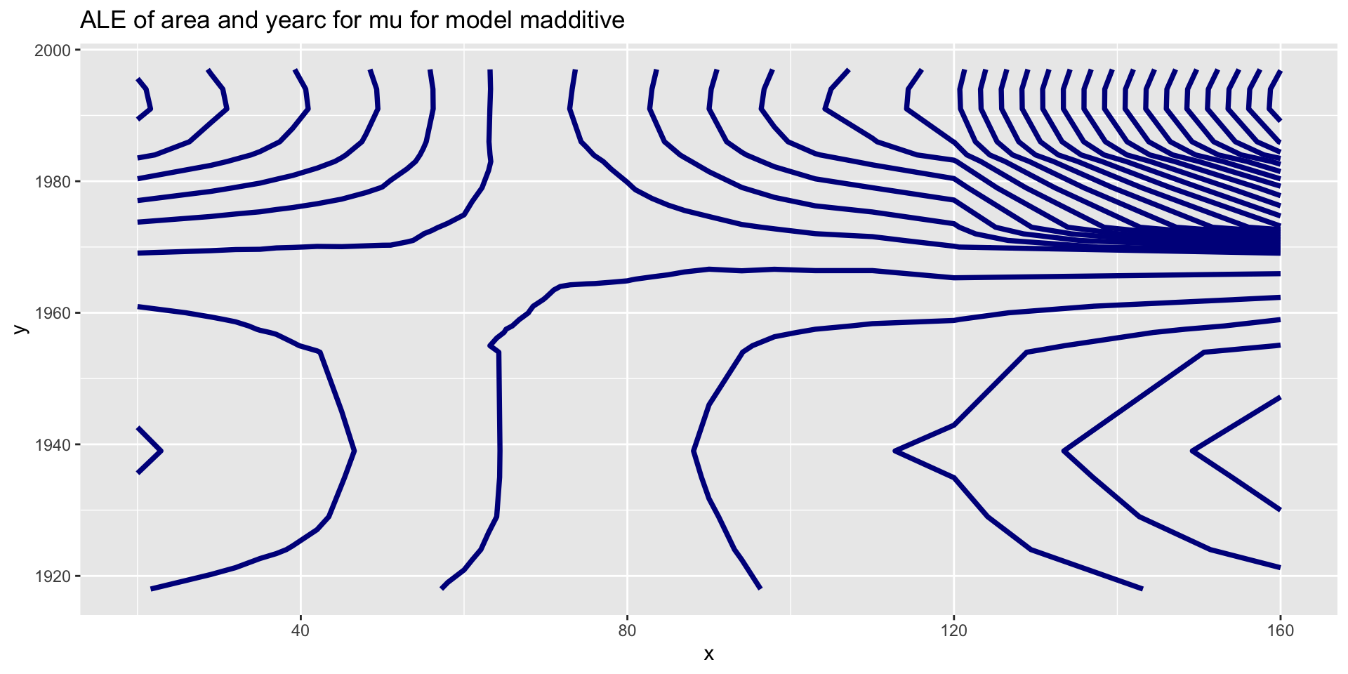
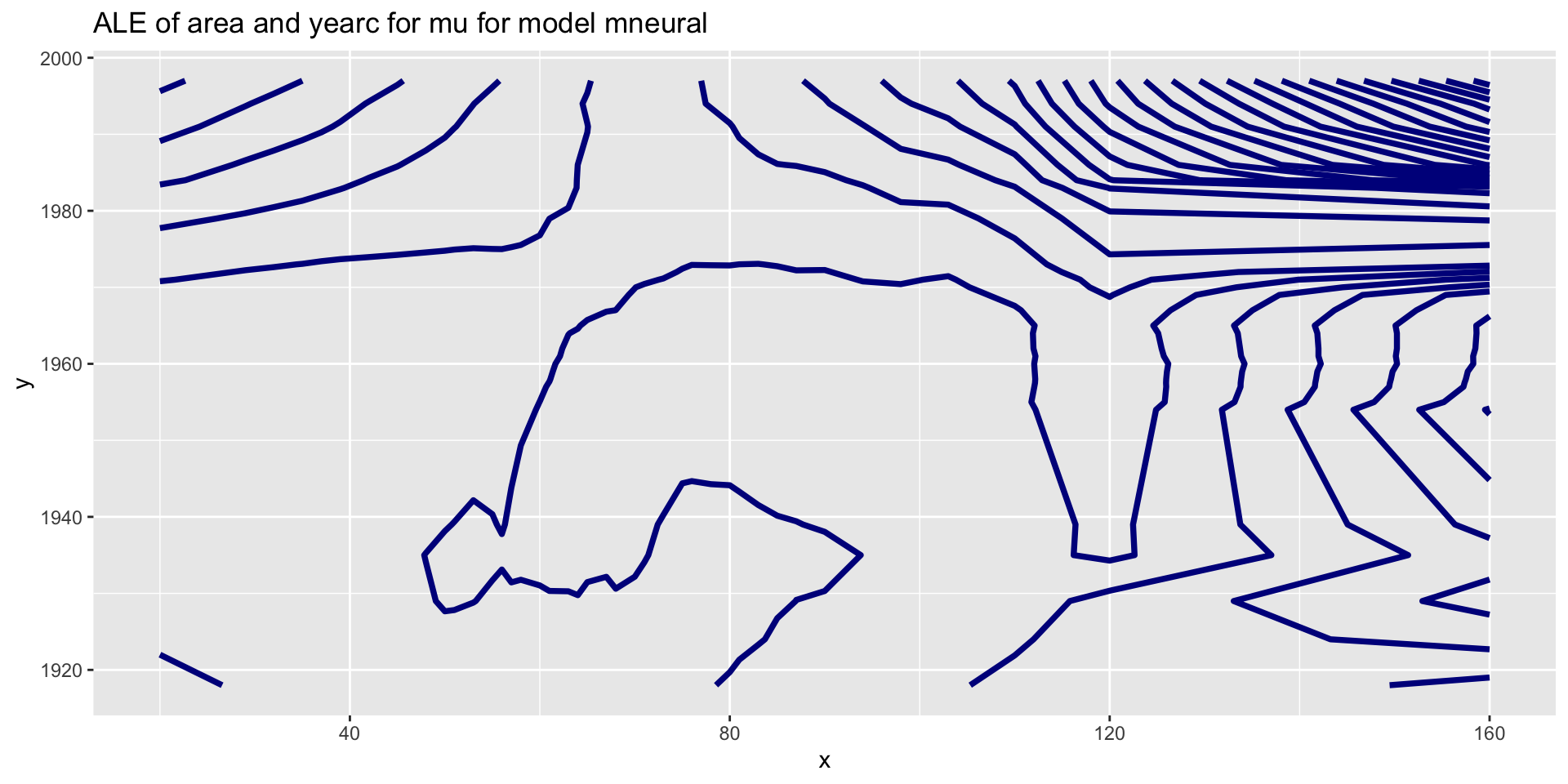
ALE interactions

gamlss.ggplots:::ale_param(madditive,c("area", "yearc"))
gamlss.ggplots:::ale_param(mneural,c("area", "yearc"))
moments (mean)

  • Not implemented yet for gamlss2 objects

  • Note that moments not always exist for example for the BCTo distribution

    • for \(\tau\le2\) the variance do not exist

    • for \(\tau\le1\) the mean do not exist

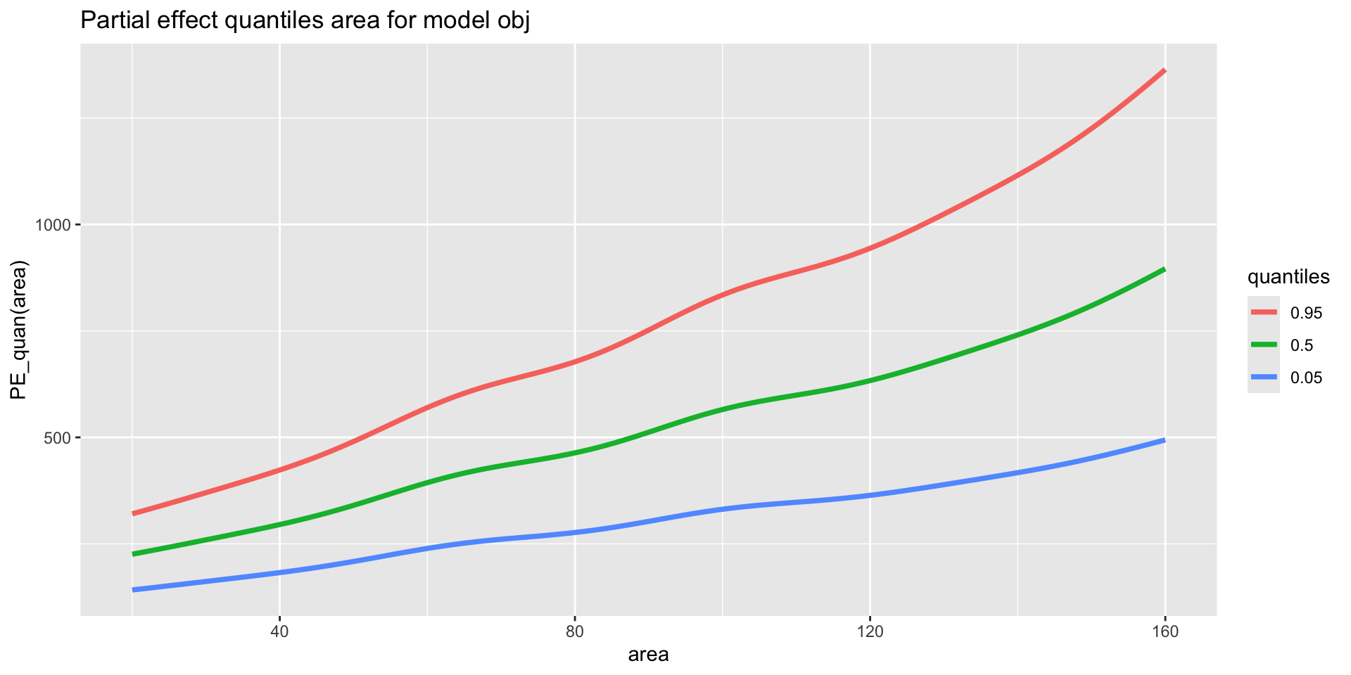
quantiles, additive

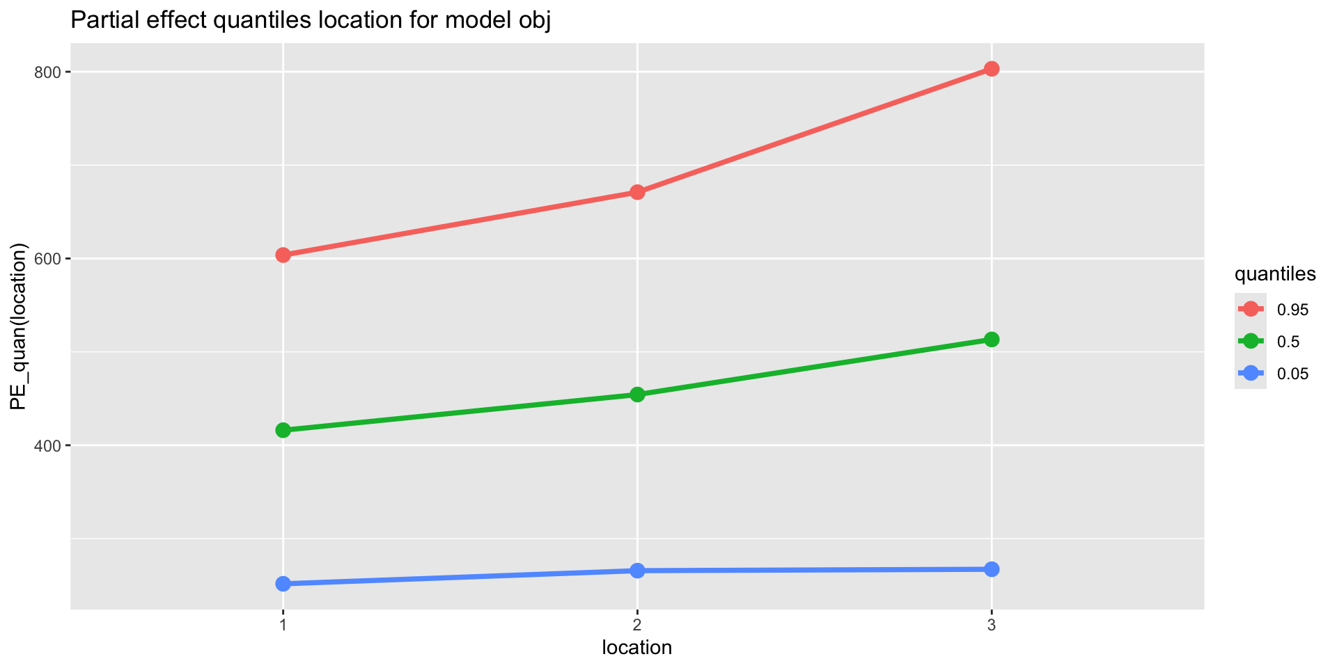
 gamlss.ggplots:::pe_quantile(madditive,c("area"))

quantiles, additive (con.)

quantiles interactions
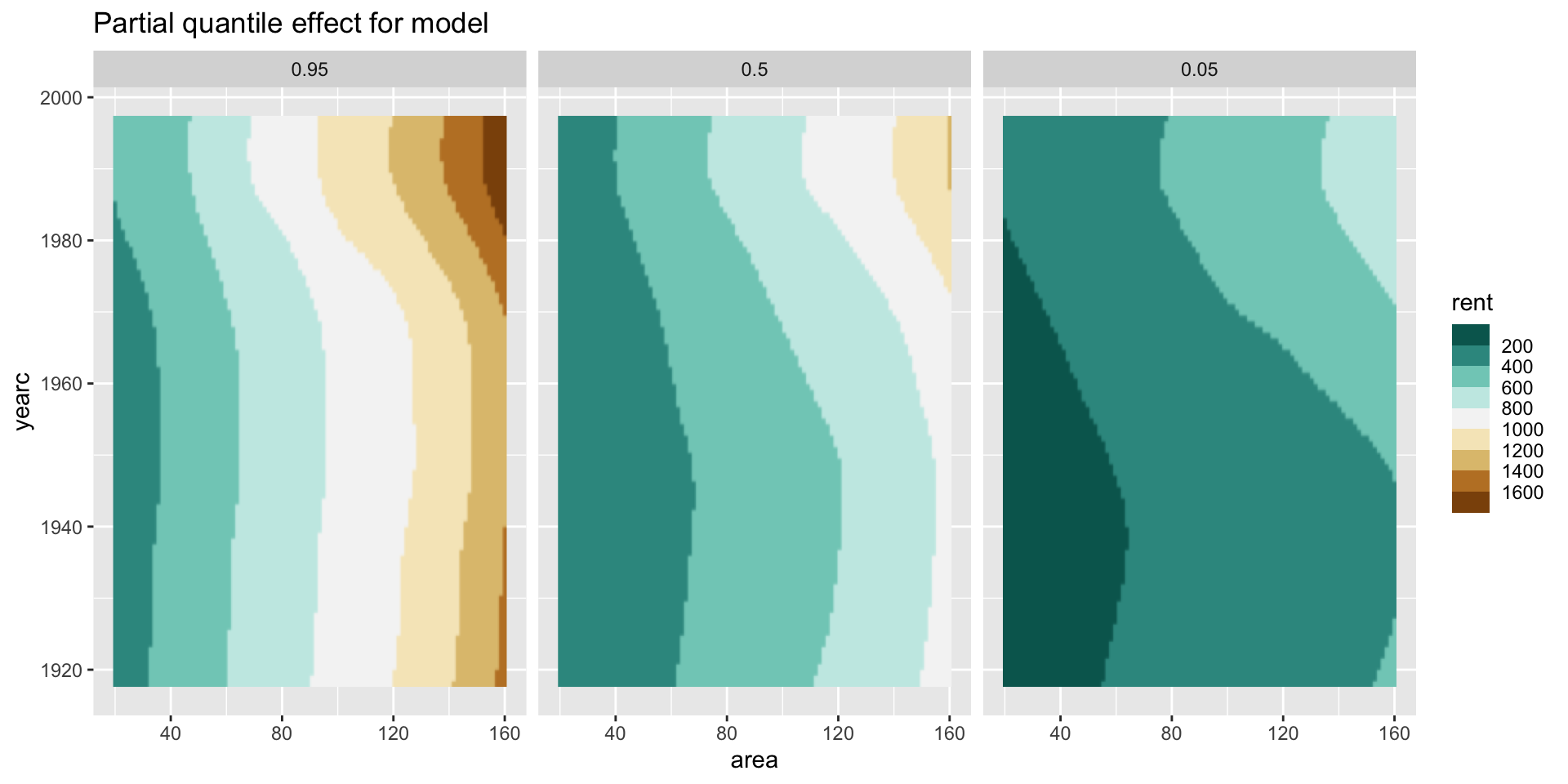
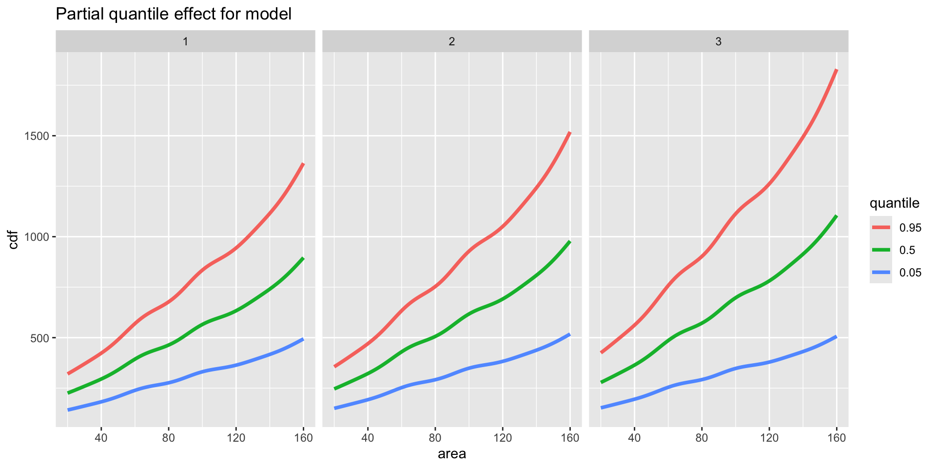
  gamlss.ggplots:::pe_quantile(madditive,c("area", "yearc"))

quantiles interactions 2

 gamlss.ggplots:::pe_quantile(madditive,c("area", "location"))

quantiles interactions 2

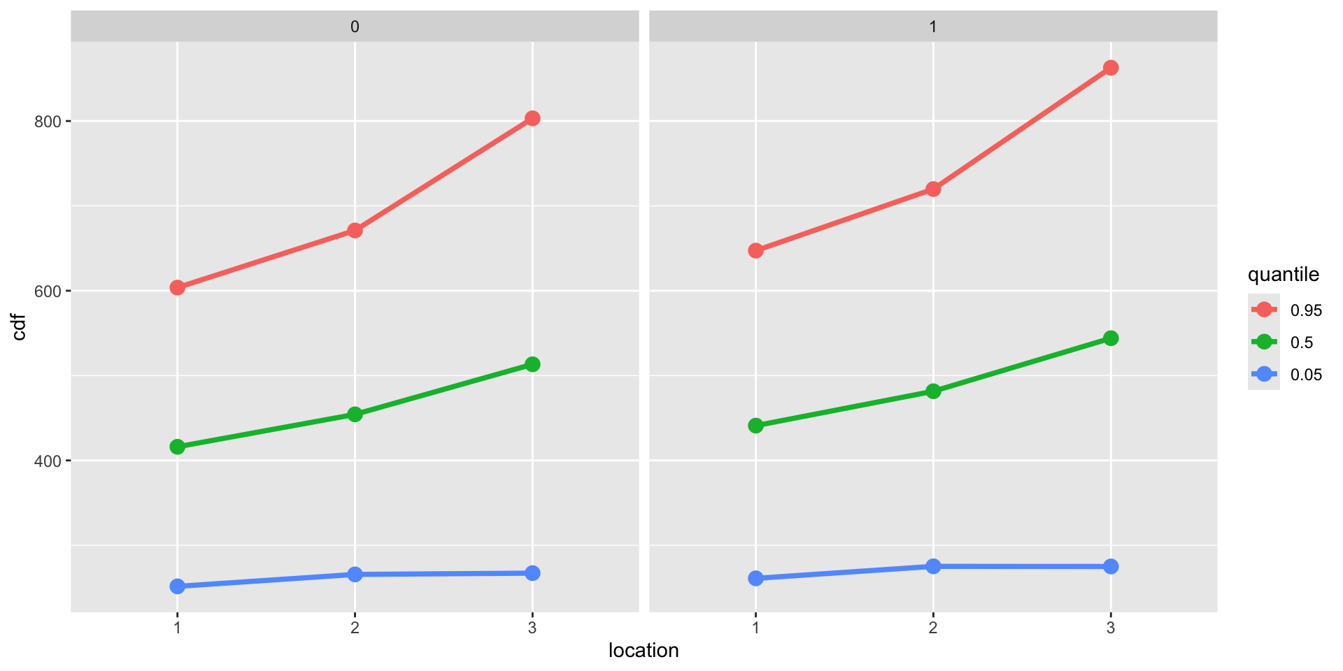
gamlss.ggplots:::pe_quantile(madditive,c( "location", "bath"))

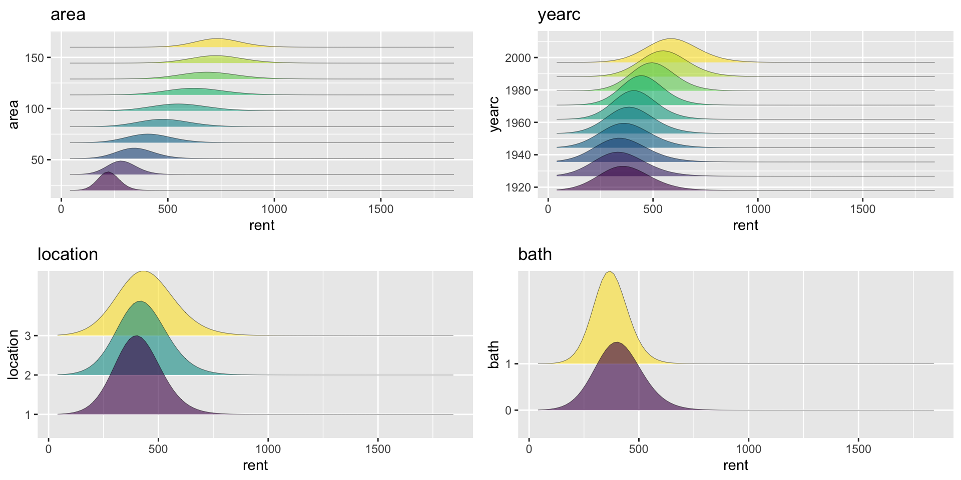
distributions, \(\mu\), additive

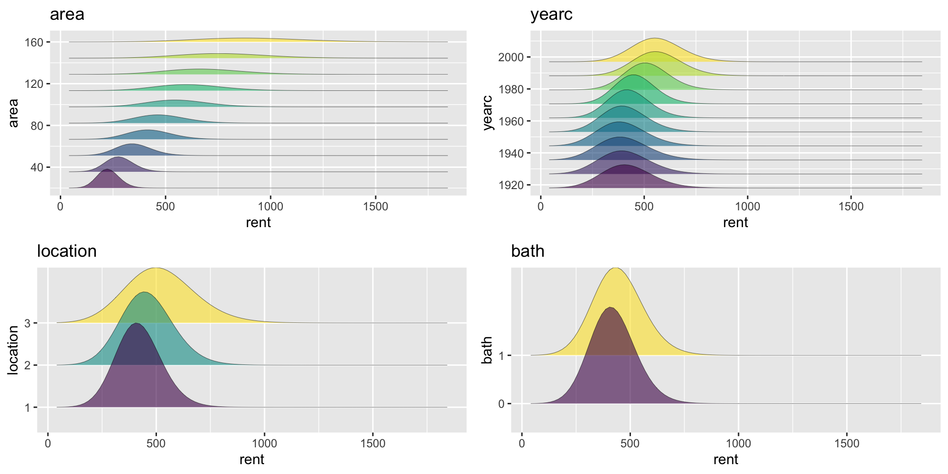
gamlss.ggplots:::pe_pdf_grid(madditive, list("area", "yearc", "location","bath"))

distributions, \(\mu\), NN

gamlss.ggplots:::pe_pdf_grid(mneural, list("area", "yearc", "location","bath"))

the purpose of the study

  • the purpose should be always in our mind when we try to analyse any data

  • for the Munich rent data are collected almost every 10 years

  • guidance to judges on whether a disputed rent is a fair or not

  • purpose is to identify very low or very hight rents by correcting for the explanatory variables

  • similar in detecting “outliers”

  • a possible solution: prediction z-scores

prediction z-scores

Scenarios

rent area yearc location bath kitchen heating
1500 140 1983 3 1 1 1
1000 55 1915 1 0 0 0
800 65 1960 1 1 1 1

prediction z-scores (con.)

     rent <- c(1500, 1000,800)
     area <- c(140, 55, 65)
    yearc <- c(1983, 1915, 1960)
 location <- factor(c(3,1,1))
     bath <- factor(c(1,0,1))
  kitchen <- factor(c(1,0,1))
 cheating <- factor(c(1,0,1))
 ndat <- data.frame(rent, area, yearc, location, bath, kitchen, cheating)
 cat("prediction z-scores", "\n")
prediction z-scores 
 pp <-predict(madditive, newdata=ndat, type="parameter")
  qNO(madditive$family$cdf(q=ndat$rent, par=pp))
[1] 0.2616374 4.7737859 2.0955995

summary

GAMLSS can tackle problems where the interest of the investigation lies not only in the center but other parts of the distribution.

Personal view for the future of GAMLSS development;

  • theoretical contributions

  • software and

  • knowledge exchange

Summary (continue)

  • theoretical contributions
    • interpretable tools
    • model average for prediction
  • software
    • gamlss2
  • books and knowledge exchange
    • there is need for applied and elementary books
    • more application public health and environment

the team

working party current past
Gillian Heller Konstantinos Pateras Popi Akantziliotou,
Fernanda De Bastiani Paul Eilers , Kevin Burke Vlasios Voudouris, Nadja Klein
Thomas Kneib Nikos Kametas Marco Enea, Nicoleta Mortan
Achim Zeileis Tim Cole Daniil Kiose, Florian Ziel
Andreas Mayr Artur Fredrich Dea-Jin Lee, Peru Muniain
Nicolaus Umlauf Luiz Nakamura María Xosé Rodríguez-Álvarez
Reto Stauffer Elisa Van Eynde Majid Djennad
Robert Rigby Julian Merder Nikos Georgikopoulos
Mikis Stasinopoulos Abu Hossain Raydonal Ospina, Fiona McElduff

end

back to the index

The Books