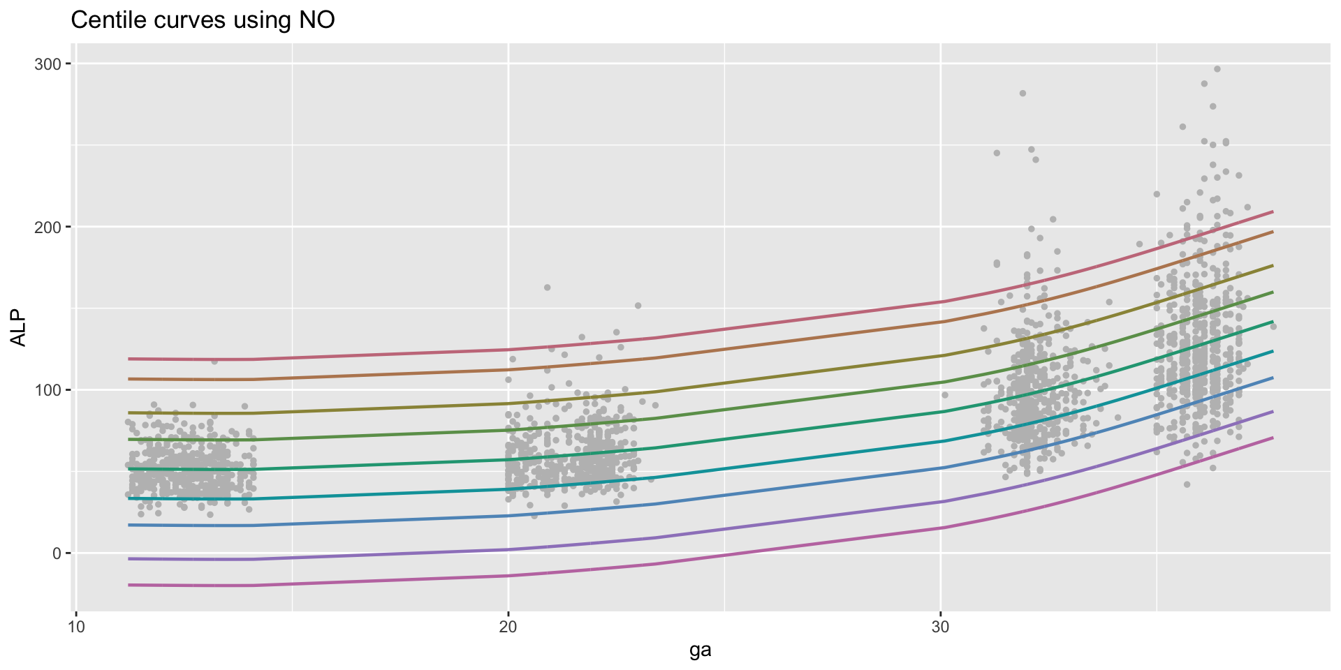

GAMLSS-RS iteration 1: Global Deviance = 19556.8715 eps = 0.069510
GAMLSS-RS iteration 2: Global Deviance = 19556.8715 eps = 0.000000
how to adapt for climate change challenges
machine learning models as they stand, are not always suitable for environmental data
goodness of fit measure should represent more closely the question in hand
Interpretation of the model is important for improvements in scientific knowledge
this talk is my personal opinion on how regression models should adapt for environmental data
data; used to mean a file with a lot of;
numbers, (but data today could have)text,pixels, orinformation.data analysis is the art of extraction information from the data.
Regression model deal with tabular data
| obs number | y | x1 | x2 | x3 | … | xr-1 | xr |
|---|---|---|---|---|---|---|---|
| 1 | y1 | x11 | x12 | x13 | … | x1r-1 | x1r |
| 2 | y2 | x21 | x22 | x23 | … | x2r-1 | x2r |
| 3 | y3 | x31 | x32 | x33 | … | x3r-1 | x3r |
| … | … | … | … | … | … | … | … |
| n-1 | yn-1 | xn-11 | xn-12 | xn-12 | … | xn-1r-1 | xn-1r |
| n | yn | xn1 | xn2 | xn3 | … | xnr-1 | xnr |
The size of observations \(n\) keeps growing over time
the size of the variables \(r\) is also increase
traditionally \(n > r\) but now other situations are common
there is information in data before start modelling we need to explore (see the package gamlss.prepdata)
data partition helps the model building?
data partition help with
checking for over-fitting
helping to improve inference by providing extra information about variations
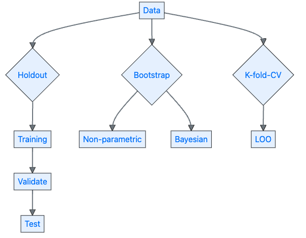
there two types of partition
single partition (holdout samples)
multiple partitions (bootstrapping, K-fold cross validation )
partition
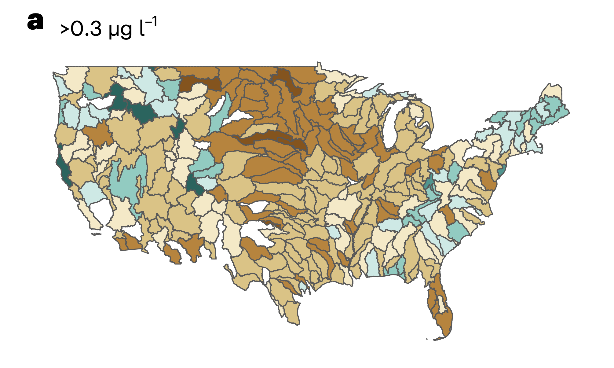
toxicity in USA lakes (Merder et al. 2023)
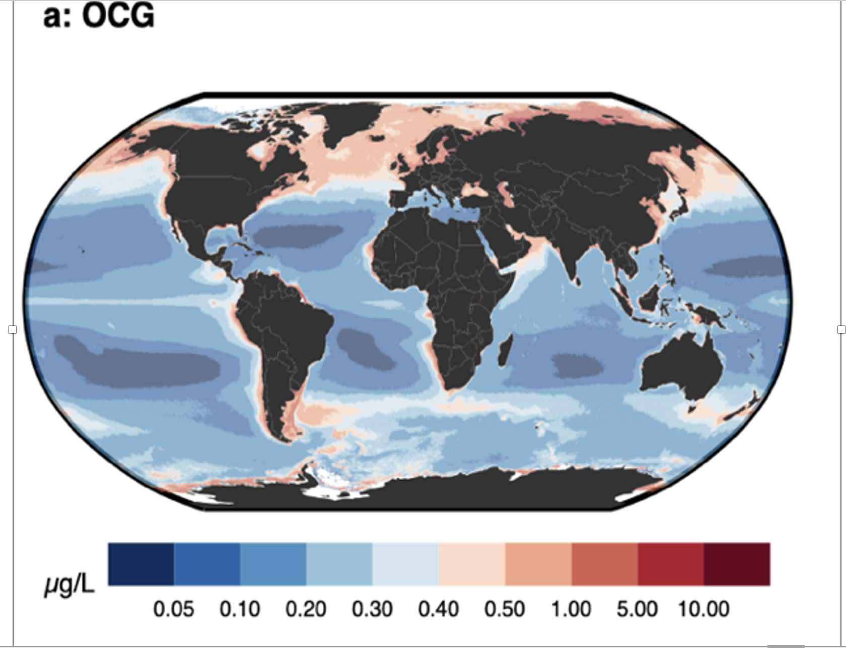
pollution in the oceans using satellite images (Merder et al. 2024)
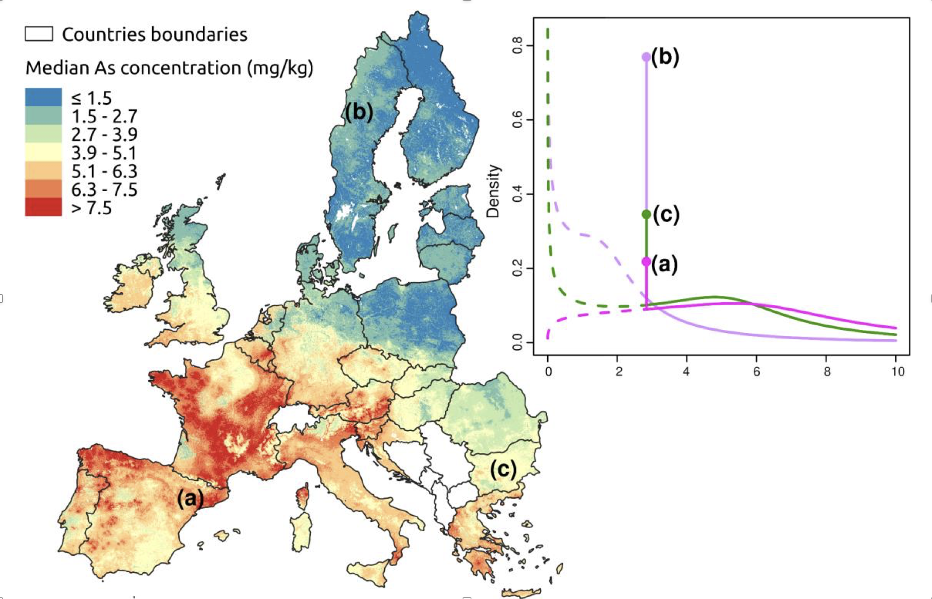
arsenic in EU soil see (Fendrich et al. 2024)
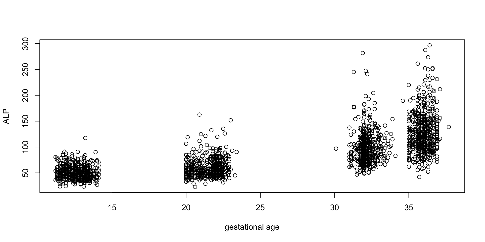
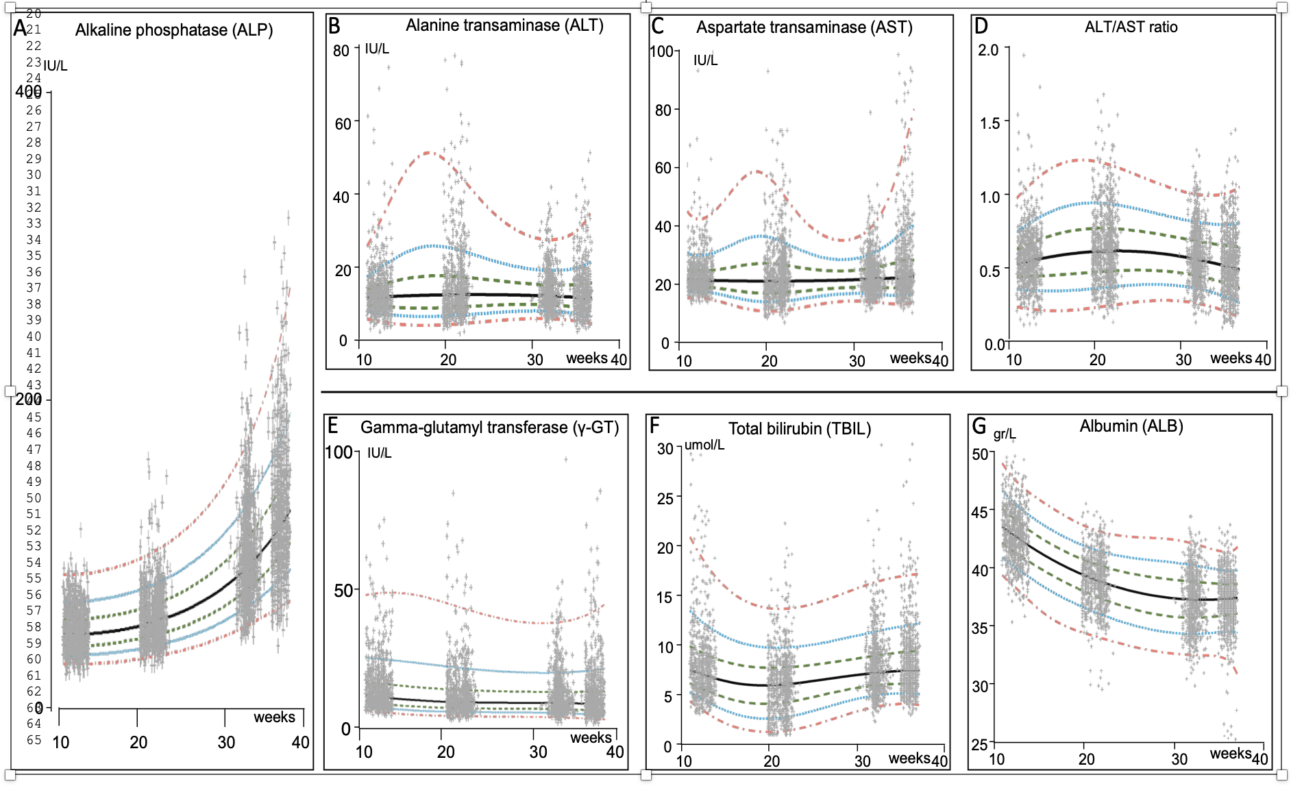
monitor liver functions during pregnancy (Judah et al. 2025)
phosphorus in the soil in EU (current work)
the response is ALP Alkaline Phosphatase an enzyme found throughout the body, but especially in: Liver, Bones, Kidneys, Intestines, Placenta (during pregnancy)
the x-var is gestation age
To analyse data we use models.
a model is a simplification of reality.
toy models, 
fashion models 
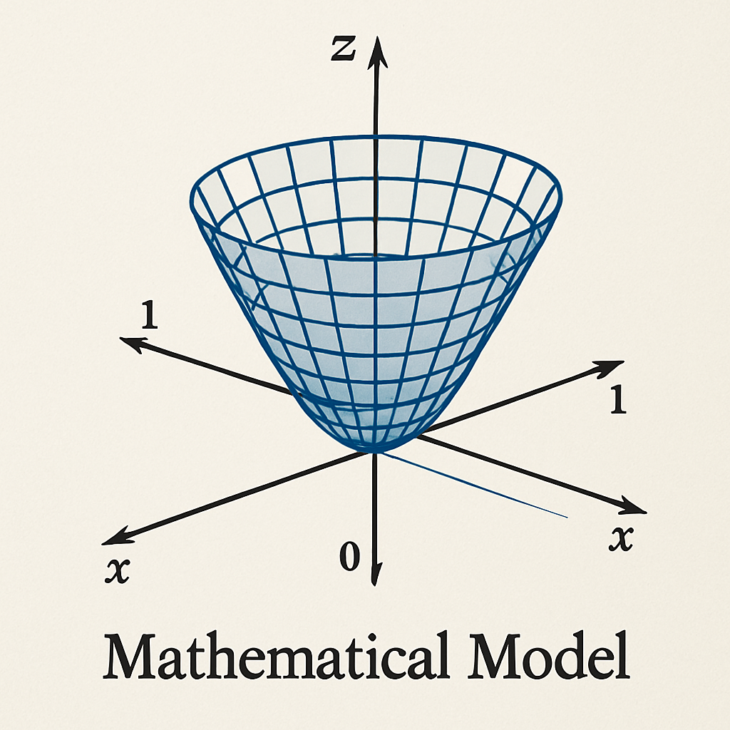
mathematical models.
where mathematical equations are used to describe reality.
all models are wrong but some are useful.– George Box (1979)
whether a model is useful depends on the purpose of the study.
is the model adequate to answer the question?
the question is the hypothesis, the purpose of the study; It is what the researcher tries to understand and answer
the next question is:
can the data or the model answer the question in hand?
if the answer is yes then how.
can be answered by regression analysis?
regression is an input-output model.
we have information on variable(s) \(X\), the input variables,
and we want to use this information to say something about the variable(s) \(Y\) the output.
Input-output model are supervised learning model (since a response variable exist)
Breiman (2003)
\[ X {\longrightarrow} \fbox{NATURE} {\longrightarrow} Y, \ \textit{(complex)} \]
\[ X {\longrightarrow} \fbox{Model} {\longrightarrow} Y \ \textit{(simpler)} \]
\[ X {\longrightarrow} \fbox{f()} {\longrightarrow} Y \ \textit{(mathematical model)} \]
the task is to unmask the unknown function \(f()\).
a compete unspecified function lead to AI otherwise we rely on assumtions
an assumption is an axiomatic statement which need to be accepted for the model to work.
the reasoning is that: if the assumptions are correct then the model should be OK
mathematical assumptions also help intepretation of a model i.e.
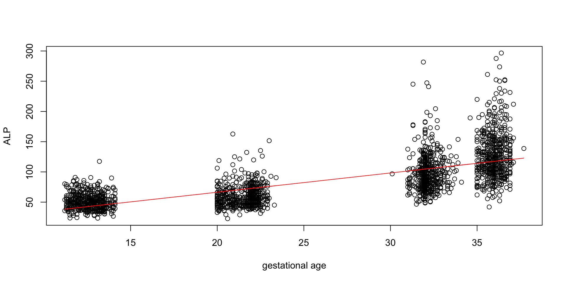
linear assumption for \(f()\) is \(\alpha+\beta_1 x_1 + \ldots + \beta_p x_p\)additive assumption for \(f()\) is \(\alpha+f_1(x_1) + \ldots + f_p(x_p)\)GAMLSS-RS iteration 1: Global Deviance = 19556.8715 eps = 0.069510
GAMLSS-RS iteration 2: Global Deviance = 19556.8715 eps = 0.000000
\(ALP \sim NO(\mu,\sigma)\)
\(\mu=\alpha +\beta \: \text{ga}\)
\(\sigma\)= constant
\(ALP\) observations are independent
GAMLSS-RS iteration 1: Global Deviance = 19305.9535 eps = 0.081448
GAMLSS-RS iteration 2: Global Deviance = 19304.412 eps = 0.000079
GAMLSS-RS iteration 3: Global Deviance = 19304.4115 eps = 0.000000
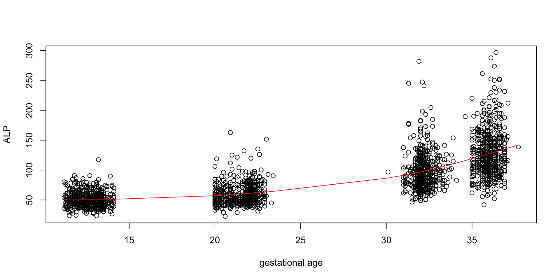
explicit assumptions, usually mathematical, are easy to check
implicit assumptions (more difficult to check)
incorrect assumptions could lead to questionable scientific discoveries
we should check explicit assumptions using diagnostic tools
algorithmic models make mostly implicit assumptions about the function \(f()\).
an algorithmic model is a step-by-step computational procedure designed to perform a task by systematically transforming inputs into outputs according to a defined set of rules.
no explicit assumptions for \(f()\) are needed but a lot of implicit assumptions depending on the algorithm
algorithmic models (like mathematical models) can be deterministic or stochastic
a stochastic model is a (mathematical or algorithmic) model which incorporates randomness so its output is not completely predictable even with the same starting conditions.
stochastic regression models contain probabilistic assumptions on how the input-output model is generated.
the minimal assumption for a regression model is about the behaviour of the response
in linear models \(\textbf{y}=\textbf{X}\boldsymbol{\beta}+e\) where \(e_i \sim N(\boldsymbol{0}, \sigma^2)\) is the classical stochastic model.
not all problems need a stochastic component
Stochastic models are often used because many natural, social, and physical systems have inherent variability.
a stochastic algorithmic model is often called a machine learning model
a typical supervised machine learning model has the form \[Y= g(X)+ \epsilon\] where the error \(\epsilon\) is assumed to be an identical and independently distributed random variable
implicitly it is assumed that the error is a symmetrical random variable.
input-output model can be written as\[
X {\longrightarrow} \fbox{f()} {\longrightarrow} E(Y)
\] where the \(E(y)\) is the expected value of \(Y\) plus
implicit assumptions for \(f()\) and
explicit symmetrical and independent assumption for \(\epsilon\)
only the mean is modelled
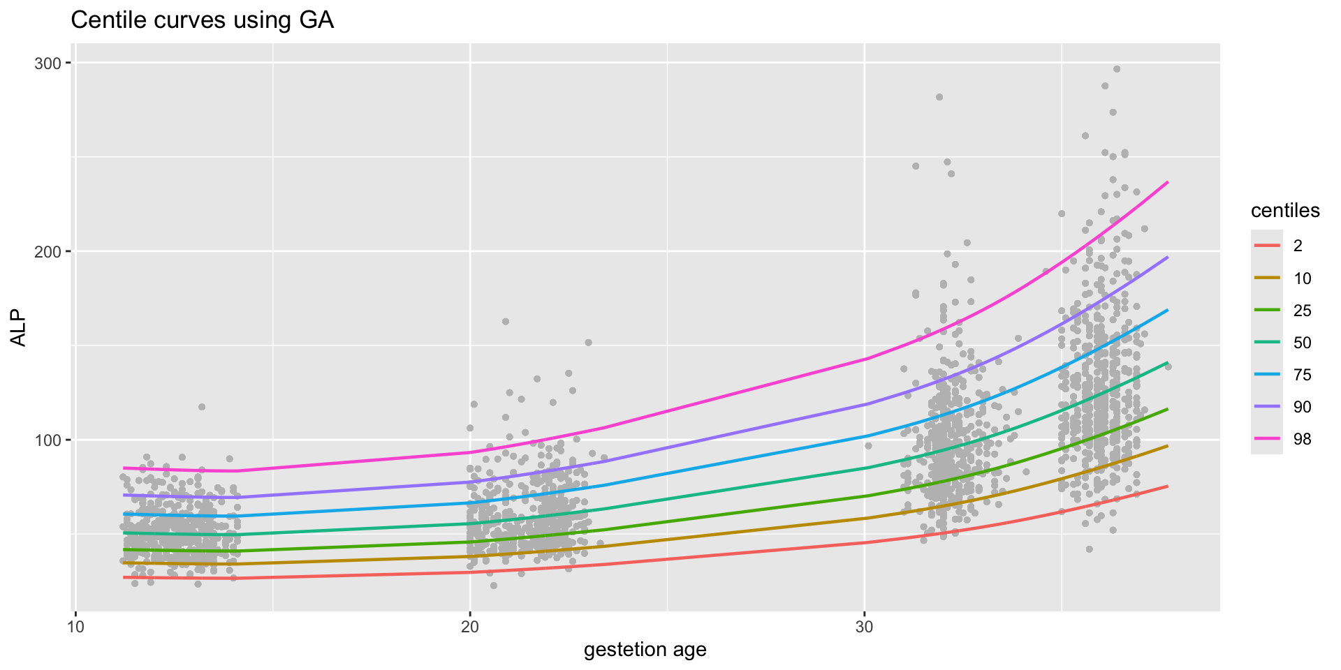
\(ALP \sim NO(\mu,\sigma)\)
\(\mu= f(\text{ga})\)
\(\sigma\)= constant
\(ALP\) observations are independent
all are implicit assumptions that some machine learners forget or do not bother to tell
GAMLSS-RS iteration 1: Global Deviance = 18752.8733 eps = 0.107763
GAMLSS-RS iteration 2: Global Deviance = 18680.5714 eps = 0.003855
GAMLSS-RS iteration 3: Global Deviance = 18680.5446 eps = 0.000001
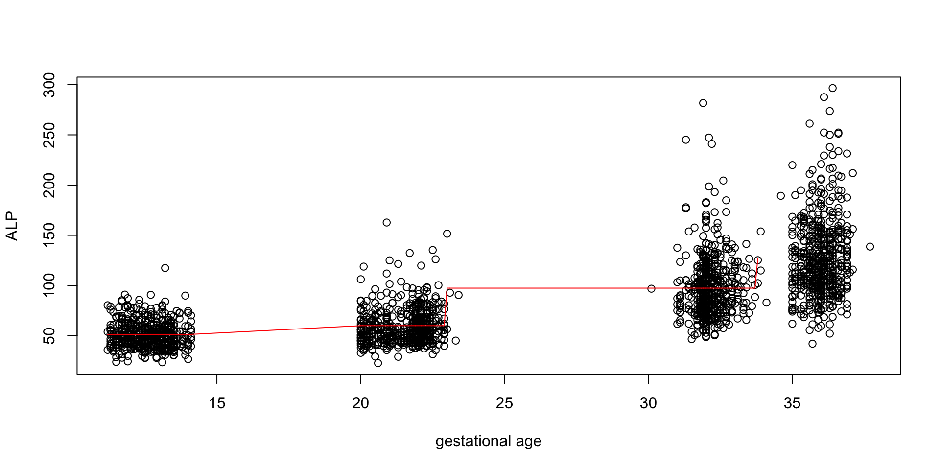
algorithm models could be black box’s
they are two main reasons for a black box
the function \(f()\) is too complicated to explain
there are proprietary reasons
black box against interpretable
transparent, explainable, comprehensive models
the question in hand should determine whether the model should be interpretable.
“Stop explaining black box machine learning models for high stakes decisions and use interpretable models instead” (Rudin 2019)
the argument came from the fact that among all adequate models (the Rashomon set) few are interpretable (Rudin et al. 2024)
GAMLSS-RS iteration 1: Global Deviance = 19395.3504 eps = 0.077195
GAMLSS-RS iteration 2: Global Deviance = 19342.6355 eps = 0.002717
GAMLSS-RS iteration 3: Global Deviance = 19341.3729 eps = 0.000065
GAMLSS-RS iteration 4: Global Deviance = 19341.3725 eps = 0.000000
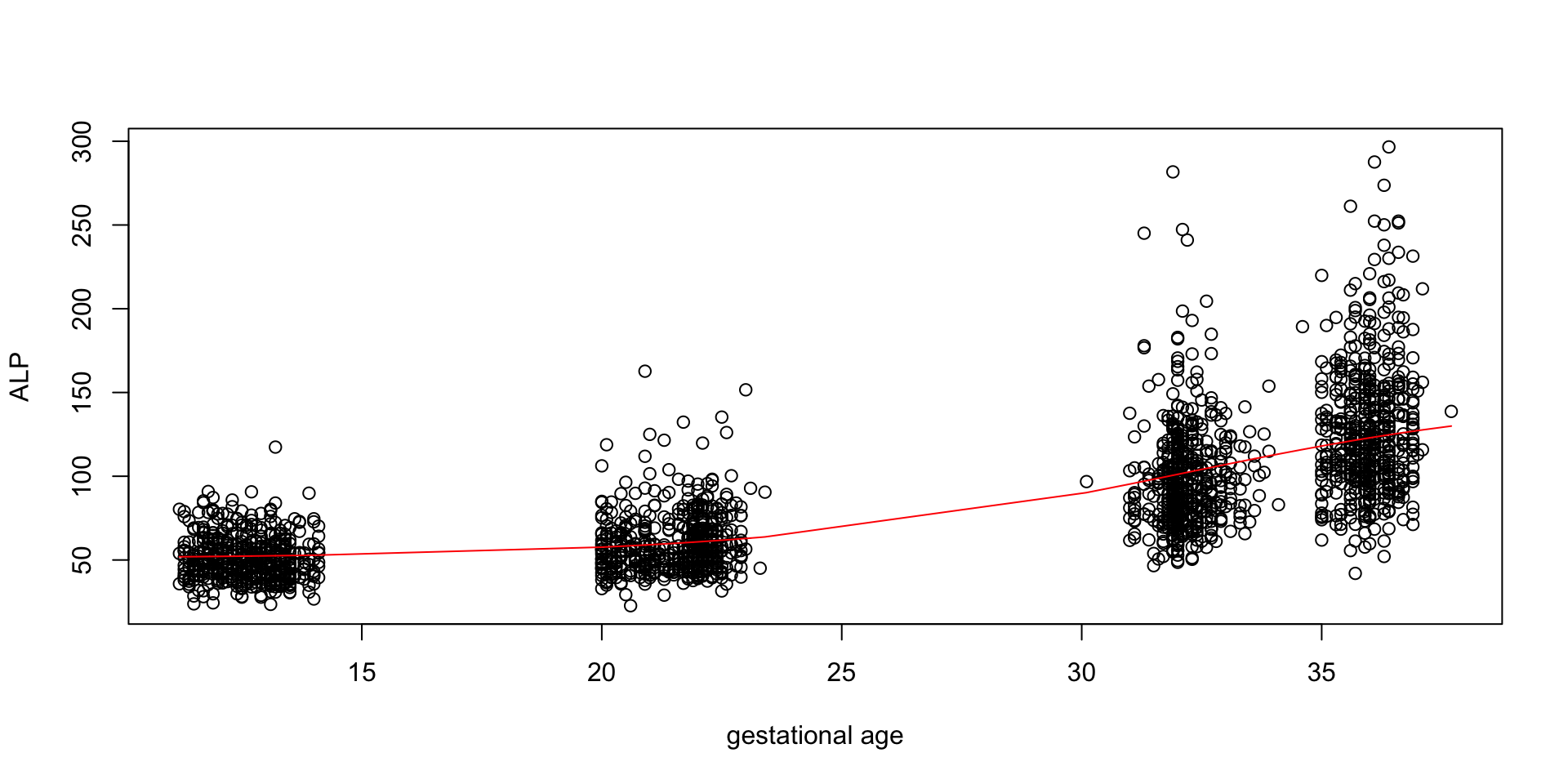
GAMLSS-RS iteration 1: Global Deviance = 19296.2132 eps = 0.081912
GAMLSS-RS iteration 2: Global Deviance = 19294.2941 eps = 0.000099
GAMLSS-RS iteration 3: Global Deviance = 19294.2941 eps = 0.000000
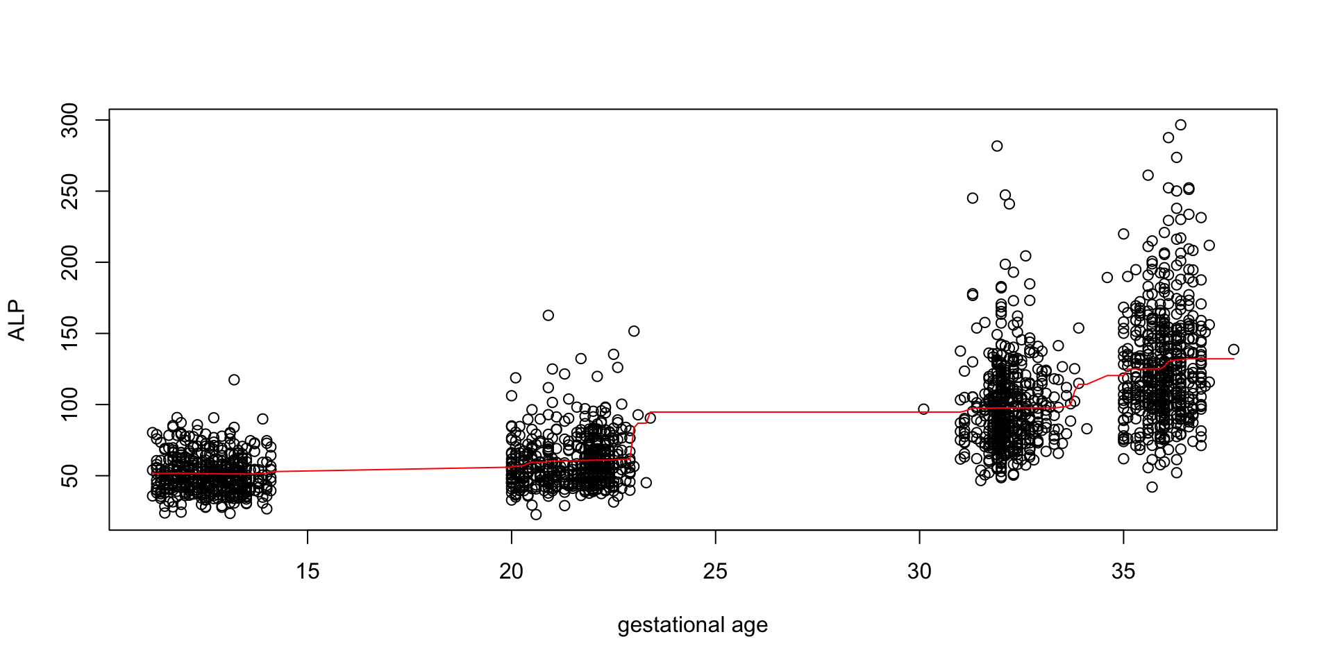
data
assumptions
model
mathematical or algorithmicinterpretable or black boxHow we can compare the accurancy between different models?
this is done usually using a risk function
A risk function measure the accuracy of the model. [it measure how accurate \(f()\) is for a specific risk function]
a risk is defined as the expected loss \(\ell\). That is, we define a lost function \(\ell\) first as a function of the response \(Y\) and the explanatory variable \(X\) and then we take expectations: \[R(f) = \mathbb{E}_{X,Y} [ \ell(g(X), Y) ]\] -\(g()\) is the model,
squared error : \((y_{true} - y_{fitted})^2\)
absolute error: \(\left|y_{true} - y_{fitted} \right|\)
information based error: \(- \int_{-\infty}^\infty f_{true}(y|x) \log f_{fitted}[y, \theta(x) ] dy\)
risk functions could include penalty terms
empirical risk: instead of taken expectation using the unknown true distribution we just average over the observations i.e. \(\frac{1}{n} \sum_{i}^{n} (y_{true,i} - y_{fitted,i})^2\)
the empirical risk is the log likelihood for information based measure
the evaluation of the empirical risk is more effective if it is done on out of bag data, or test data
the square error and absolute error risk functions tell us how far the \(Y\) is from its estimated expected value \(E(Y)\). They tell us nothing on how well other part of the distribution for \(Y\) are fitted i.e. the tails
the empirical risk should be always related to the question in hand.
information based criteria:
AIC df
Reg_Tree 18704.54 12.000000
Add_Mod 19315.91 5.749771
NN_Mod 19407.37 33.000000
Ran_For 19498.29 102.000000
Lin_Mod 19562.87 3.000000
AIC df
Reg_Tree 18772.05 12.000000
Add_Mod 19348.26 5.749771
Lin_Mod 19579.75 3.000000
NN_Mod 19593.02 33.000000
Ran_For 20072.10 102.000000
the degrees of freedom of the model is a measure of model complexity
for mathematical models the df’s are the number of parameters fitted in the model
for algorithmic models the df’s are difficult to define
data are separated to training and test data sets
Mean Square Error (test observations)
models MSE
[1,] "Add_Mod" "726.698"
[2,] "NN_Mod" "728.525"
[3,] "Ran_For" "730.387"
[4,] "Reg_Tree" "738.687"
[5,] "Lin_Mod" "796.054"
test observations) models MAE
[1,] "Add_Mod" "18.9538"
[2,] "Ran_For" "19.0120"
[3,] "NN_Mod" "19.0525"
[4,] "Reg_Tree" "19.0789"
[5,] "Lin_Mod" "20.4588"
deviance \(-2 \log Likelihood\) (test observations)
models pdeviance
[1,] "Reg_Tree" "12518.98"
[2,] "Add_Mod" "12904.79"
[3,] "NN_Mod" "12908.19"
[4,] "Ran_For" "12911.92"
[5,] "Lin_Mod" "13029.86"
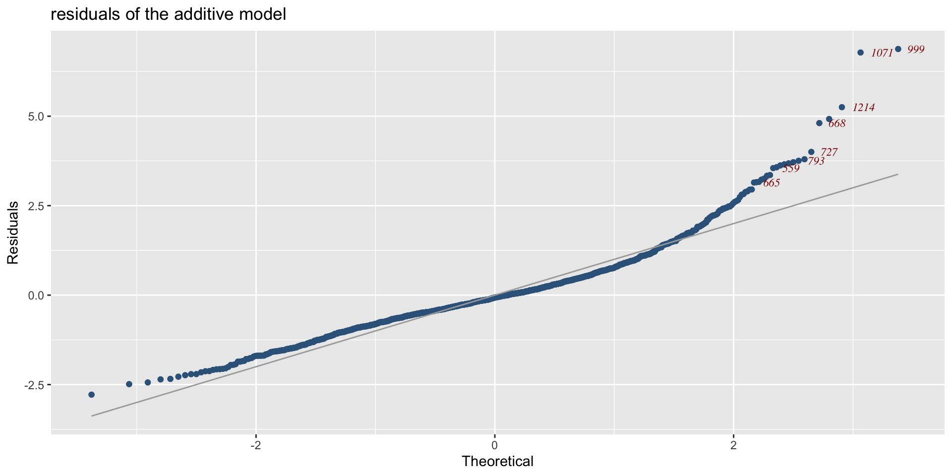
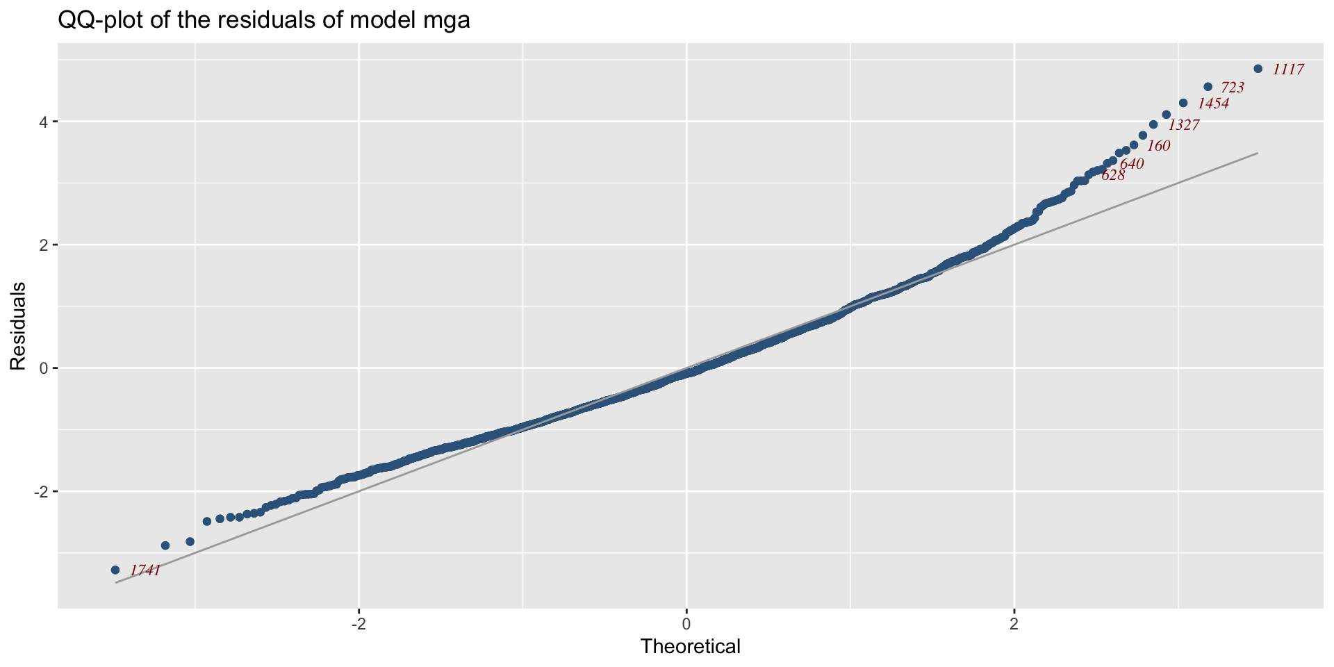
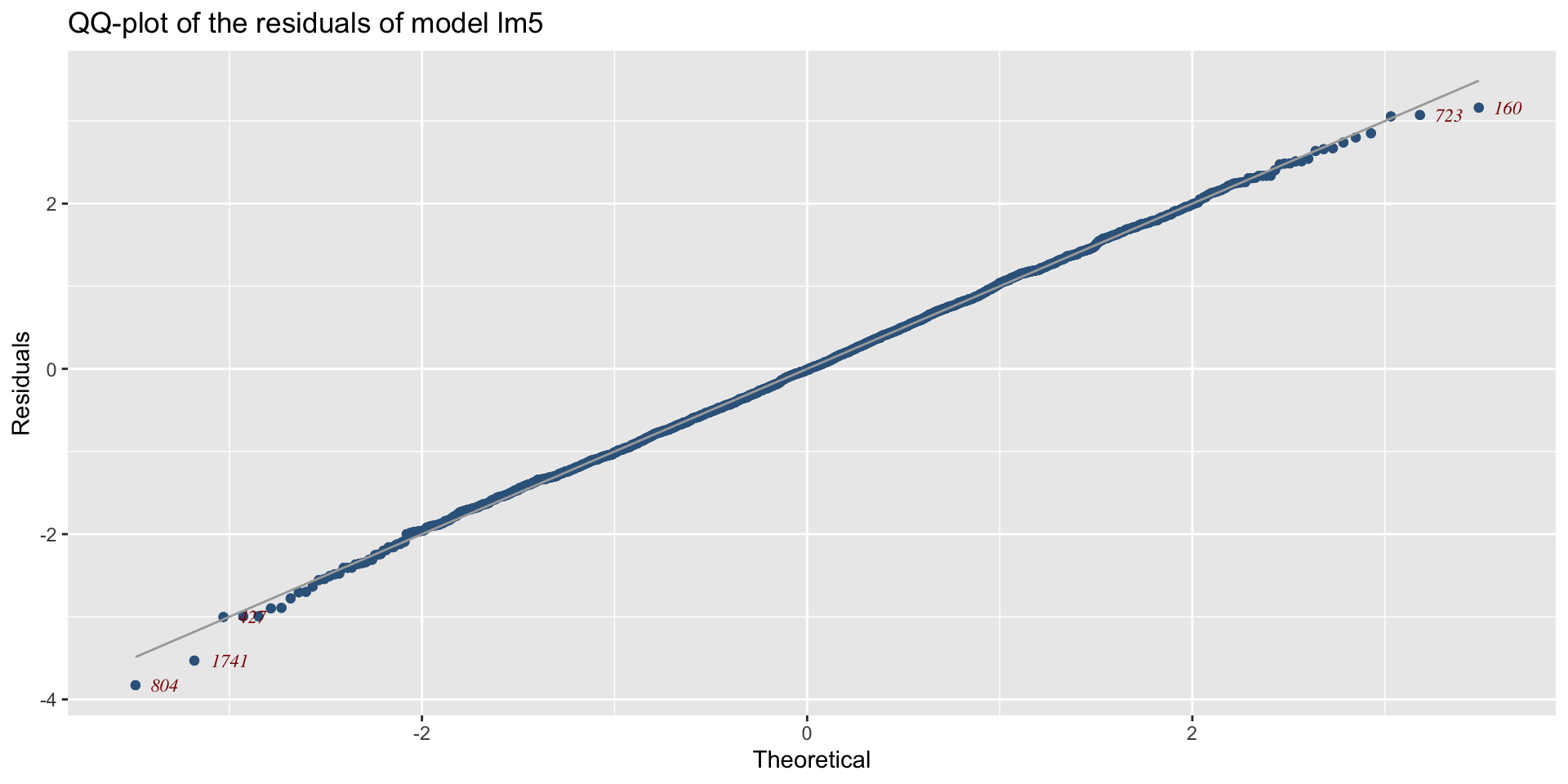
in order to produce the predictive deviance results we assume that the distribution for the response is normal.
Is this a sensible assumption?
let us test it
input-output model it can be written as \[
X {\longrightarrow} \fbox{f()} {\longrightarrow} E(Y)
\] where \(g()= g(\eta=\textbf{X}\boldsymbol{\beta})\) and \(g()\) is called a link function to make sure that values of \(\mu=E(Y)\) are in the right rangewhere D() is a distribution belonging to the exponential family
- normal, gamma, inverse Gaussian
- Poisson, bimomial
\(g(\boldsymbol{\eta})\) allows only linear effects [for non-linear use Generalised Additive Models, GAM’s Hastie and Tibshirani (1990)]
interactions between terms have to be declared explicitly but for large number of explanatory variables this could be difficult.
Note that some ML models fit interactions as part of their algorithm i.e. regression trees, neural networks
exponential family has nice theoretical properties for the mean of \(y\), \(\left[ E(y) \right]\)
if a second parameter \(\phi\), exist it is treated as a nuisance
by ignoring \(\phi\) we have problems with:
heterogeity and over/under-dispersion
skewness and kurtosis (because are fixed)
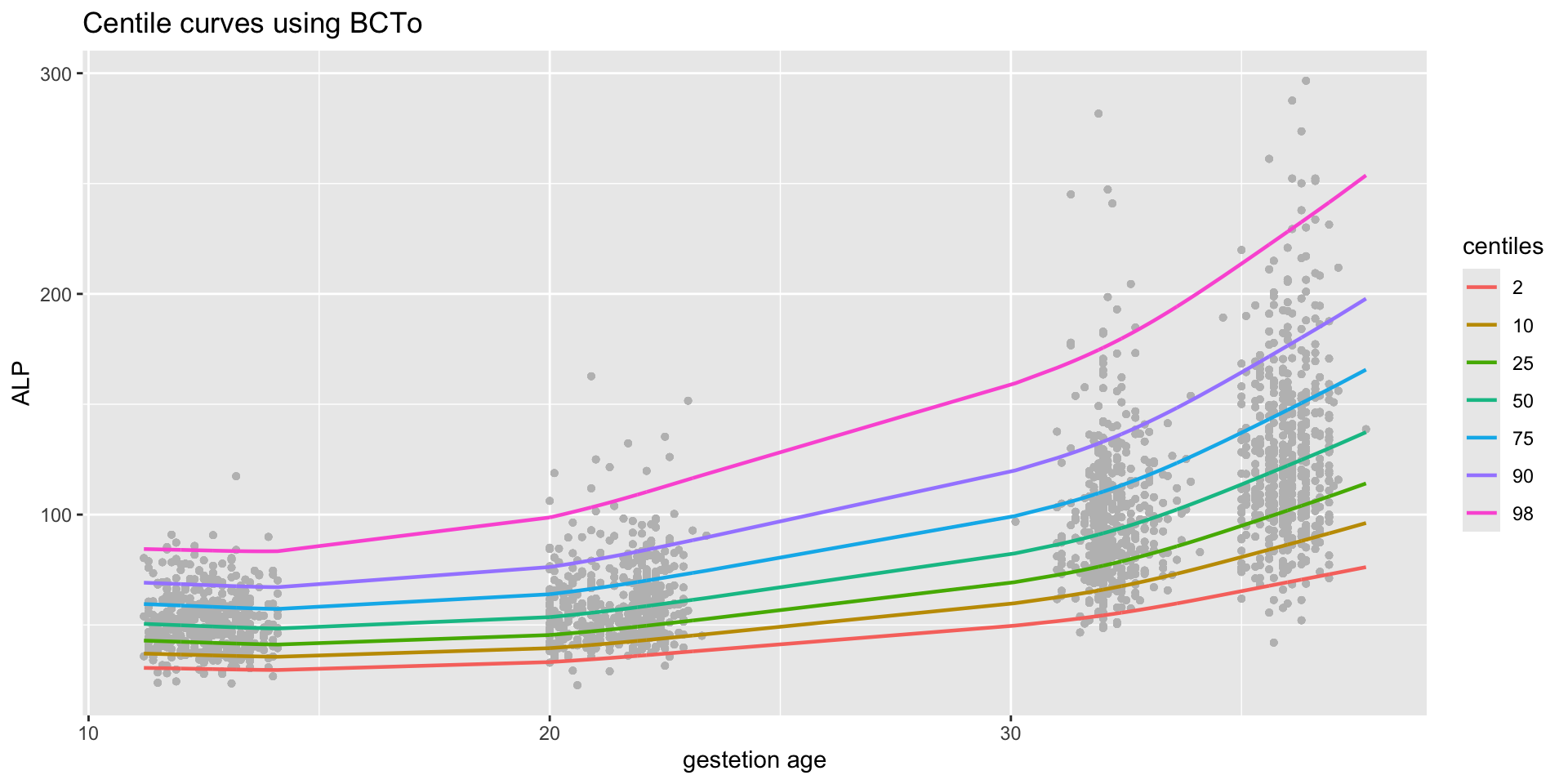
distributional regression like GAMLSS can correct those problems
Rigby and Stasinopoulos (2005) \[X {\longrightarrow} \fbox{$\boldsymbol{\theta}$()} {\longrightarrow} D(Y|\boldsymbol{\theta}(X)),
\] where \(D(Y|\boldsymbol{\theta}(X))\) represents the natural error distribution of \(Y\) (conditional on the \(X\)).
The task of Distributional Regression is to find ;


the data, the model, the question are interrelated, you can not consider one without the other in order to extract the right information.
if the question does not involve the mean of \(Y\) a GAMLSS model seems appropriate
distributional regression model could answer questions that ML and AI can not
interpretable model are important for scientific progress and easier to check using diagnostics tools
distributional regressions allows the estimation of exceedance probabilities and more generally interval forecast something that not all the classical ML model can do
distributional regression can answer questions about all aspects of the behaviour of \(Y\)
| working party | current | past |
|---|---|---|
Gillian Heller |
Konstantinos Pateras |
Popi Akantziliotou, |
Fernanda De Bastiani |
Paul Eilers , Kevin Burke |
Vlasios Voudouris, Nadja Klein |
Thomas Kneib |
Nikos Kametas |
Marco Enea, Nicoleta Mortan |
Achim Zeileis |
Tim Cole | Daniil Kiose, Florian Ziel |
Andreas Mayr |
Artur Fredrich |
Dea-Jin Lee, Peru Muniain |
Nicolaus Umlauf |
Luiz Nakamura |
María Xosé Rodríguez-Álvarez |
Reto Stauffer |
Elisa Van Eynde |
Majid Djennad |
Robert Rigby |
Julian Merder |
Nikos Georgikopoulos |
Mikis Stasinopoulos |
Abu Hossain | Raydonal Ospina, Fiona McElduff |
there are two packages in R
gamlss (older version) and
gamlss2
later version can be accessed from gamlss universe
the original paper is in web-site
The Books

www.gamlss.com